*This article introduces our AAAI-21 paper "Explaining convolutional neural networks through attribution-based input sampling and block-wise feature aggregation".

 

Emergence of "Explainable AI (XAI)"

Recently, deep neural networks (DNNs) have been successfully deployed in many fields, such as manufacturing and medicine. However, DNNs are often burdened with a large number of parameters (in the millions to tens of billions) and non-linear operations. They pose a major challenge to interpreting DNNs' behavior as to how predictions are made. AI practitioners generally consider DNNs as a "black-box" model and focus more on achieving high performance. In most cases, however, a trained model cannot guarantee its performance on out-of-sample data (i.e., data not used for fitting the model) due to its bias to the training dataset. The model bias should be assessed early on, but it is not easy to do so if the model's behavior cannot be clearly interpreted.

A research field has emerged to give high-level explanations of predictions made by AI models. We call it "Explainable AI (XAI)". XAI analyzes an AI model's behavior and shows what features of data have been leveraged by the AI model for predictions. XAI can be applied to a wide range of applications, such as vision inspection, time-series forecasting and text analysis.

Fig. 1 Use cases of explainable AI

In this paper, LG AI research focused on the development of an XAI method for image recognition. The objective is to find a weighted feature map that implies the reasoning of a DNN's prediction in a post-hoc manner and visualize it as a heatmap.

Existing XAI methods and limitations

Many XAI methods have been proposed in the field of computer vision. We can categorize them as follows: 1) backpropagation-based XAI, 2) class activation map (CAM)-based XAI and 3) perturbation-based XAI.

In the backpropagation-based XAI method, gradients are computed for each pixel to measure its effect on the output. However, this method is less interpretable, and lacks information about feature dependencies and their influence to the output. There are many variants of backpropagation-based XAI, including Integrated gradient^[1] and Full Gradient^[2], but they are not very interpretable(see fig. 2).

Fig. 2 Existing XAI methods and limitations

 

Class activation map (CAM)-based XAI methods, including Grad-CAM^[3], Grad-CAM++^[4] and Score-CAM^[5], utilize feature maps in the top layer of DNNs. The extracted features in the top layer are decisive for prediction. They can be exploited to locate the most influential features. However, the top layer features are often of low resolution. For example, the resolution of the feature map in the top layer is generally around 7×7 when the input image has 224×224 pixels. If the feature map is up-sampled to fit the input size, the resulting heatmap becomes blurry. Additionally, this method may highlight unrelated features because it takes into account of all feature maps from different channels in the top layer.

Perturbation-based XAI methods are divided into two categories. The first is an input sampling-based method and the second is an input optimization-based method. RISE (Randomized input sampling for explanation)^[6], one of the input sampling-based methods, makes thousands of perturbed copies of a single test image with corresponding random masks. The randomly masked images are fed into a DNN model to predict their scores for the target class of the test image. The masks are then linearly combined using the scores as weights. The masks with a high score include key features for the model prediction. However, this method is resource-intensive (e.g., approx. 8,000 forward passes), and the output heatmaps can be different every time due to the randomness in the perturbed images. Extremal perturbation^[7] is a famous input optimization-based method. It finds important features of a test image via an optimization process. However, this method may show irrelevant results if it fails to reach the global optimum.  Furthermore, its numerical optimization incurs high computational cost.

 

Introduction to Semantic Input Sampling for Explanation (SISE)

To overcome the limitations of the existing XAI methods, LG AI Research has developed a novel XAI algorithm, called "Semantic Input Sampling for Explanation (SISE)" in collaboration with Prof. Konstantinos Plataniotis at the University of Toronto. It achieves higher faithfulness and correctness than the previously mentioned XAI methods. Additionally, it takes less computation time.

This article provides a comprehensive summary of SISE. For more details, please refer to our AAAI-21 paper: "Explaining Convolutional Neural Networks through Attribution-Based Input Sampling and Block-Wise Feature Aggregation".

SISE is inspired by RISE which is a very intuitive method for generating an interpretable heatmap. However, RISE has some weaknesses, such as randomness in output heatmaps, noise from multiple channels and high computational cost.

Attribution-based input sampling

To resolve the weaknesses of RISE, SISE employs feature maps in the intermediate layers of a convolutional neural network (CNN) as perturbation masks (see Fig. 3). This helps improve faithfulness of the explanation because it uses the information extracted by the layers. In general, attribution-based methods pinpoint those pixels of an image responsible for a certain prediction. In the title of our paper, "attribution-based input sampling" refers to finding those feature maps in a CNN that are "appropriate" for being perturbation masks. To ensure the quality of output heatmaps and fast computation, we should strategically select layers and feature maps in a CNN.

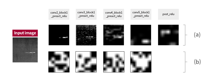
Fig. 3 (a) Examples of feature maps in intermediate layers of a CNN, (b) Examples of random masks

 

Block-wise selection

What constitutes an "appropriate" layer in a CNN can be found in (Veit, 2016)^[8]. In a nutshell, we need to identify those layers that have "much information". According to^[8], it is possible to measure the "amount of information" a layer has by removing that layer from the CNN and observing the performance degradation. As a result, the biggest drop in accuracy can be seen by removing a down-sampling layer. This shows that CNN's extracted information is refined in down-sampling layers. With this insight, SISE selects down-sampling layers.

CNNs, such as ResNet and VGG, generally perform five down-sampling operations, resulting in five down-sampling layers. Considering the sub-network between subsequent down-sampling layers as a "block", the extracted information is refined at the end of each block. The expression "block-wise" in the paper's title reflects this notion.

SISE needs to select a subset of feature maps from down-sampling layers to be computationally efficient. For example, ResNet-50 V2 has five down-sampling layers and 64, 256, 512, 1024 and 2048 feature maps in each layer. If SISE takes 4,000 feature maps, it will not be any better than RISE in terms of computational cost. SISE measures the importance of a feature map by computing the average of gradients w.r.t. pixels in that map. The maps with a positive average value become perturbation masks. This, on average, reduces the number of feature maps to below 2,000, which is less than a quarter of what RISE uses.

Feature aggregation

Selected feature maps should be combined in a proper way. To this end, SISE performs a linear combination weighted by the prediction scores of the masked inputs, resulting in a "layer visualization map" (See Fig. 4). The linear combination is carried out along each layer. Therefore, five layer visualization maps can be obtained for typical CNNs. Each map represents how the CNN deals with the input in the corresponding layer.

Fig. 4 How to aggregate selected feature maps in each layer

 

Integration of layer visualization maps

Layer visualization maps should be integrated into a heatmap for reasoning CNN's prediction. Typically, feature maps in low-level layers have higher resolution and lower SNR, whereas those in high-level layers have lower resolution and higher SNR. SISE fuses them in a cascade manner (i.e., cascade fusion) to highlight responsible features and remove noise between layer visualization maps (See Fig. 5).

Fig. 5 The cascade fusion between the layer visualization maps

 

Results of SISE

From our experiments, SISE generated a heatmap with a higher resolution than the existing XAI methods. This helped capture tiny features of small objects (See Fig. 6). This benefit could be attributed to those feature maps in the intermediate layers being the perturbation masks. As a result, SISE could more accurately and clearly identify those features relevant to CNN's prediction than the other methods which tended to yield blurry and noisy heatmaps. SISE provided consistent outputs while dealing with multiple instances from different classes (See Fig. 7).

Fig. 6 Qualitative comparison between SISE and existing methods (heatmaps testing on single object)

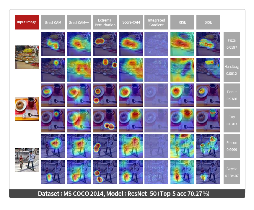
Fig.  7. Qualitative comparison between SISE and existing methods (heatmaps testing on multiple objects)

 

Two quantitative evaluations were conducted between SISE and other existing methods. The first was a ground-truth based evaluation which measured the degree of similarity between ground-truth features and XAI's prediction results. We evaluated this with the following three metrics: 1) Energy-based pointing game^[5], 2) Bounding box^[9] and 3) mIoU (mean intersection of union). The second was a model-truth based evaluation that computed the degree of faithfulness of explanations. Two metrics were considered for this: 1) Drop rate^[4] and 2) Increase rate^[4].

SISE showed better performance in the quantitative evaluations, especially it produced the state-of-the-art performance in the model-truth based evaluation (See Fig. 8).

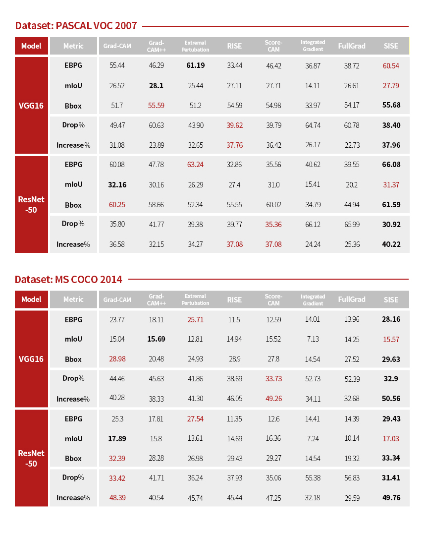
Fig. 8. Quantitative comparison between SISE and existing methods

 

Extra experiment

SISE was also evaluated on Severstal steel defect dataset^[10], an industrial dataset for visual inspection. This dataset is intended for defect detection. We modified it to use for defect classification. The modified dataset was class imbalanced; it had a limited number of defect images. The class imbalance can be commonly observed in industrial datasets because most defects occur rarely. This evaluation was designed to check if SISE would be appropriate for industrial applications. The results are given in Fig.10. SISE showed the highest faithfulness among the XAI methods. Its drop rate was significantly greater. We could clearly see that SISE could extract key features important to the CNN's prediction.

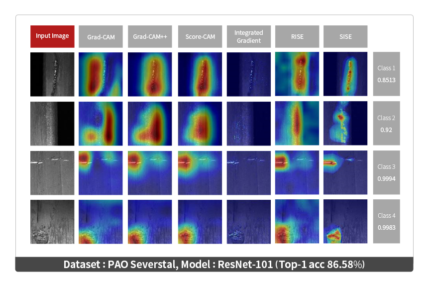
Fig. 9 Qualitative comparison between SISE and existing methods on Severstal Steel dataset

Fig 10. Quantitative comparison between SISE and existing methods on Severstal Steel dataset

 

Epilogue

SISE is a novel algorithm that can be applied to a variety of images, including those from industrial datasets for visual inspection, manufacturing and medicine. However, it is still very challenging to use XAI methods for debugging AI models. LG AI Research is developing XAI methods that can help debug and improve AI models.

Our fundamental research lab is advancing explainable AI (XAI) technologies. We intend to lead the fundamental research in XAI and accelerate its adoption to a wide range of real-world problems. To this end, our research and development for fundamental technologies will continue.

 

Acknowledgement

Special thanks to Mr. Dongsub Shim(LG AI Research Canada) for proof reading