[NeurIPS 2021] Part 3: Neural Architecture Search Review

The Conference and Workshop on Neural Information Processing Systems(NeurIPS 2021) is a machine learning and computational neuroscience conference founded in 1987. It is also one of the most influential conferences in the field of AI and machine learning with the average acceptance rate of 20%. Here is a summary of the research papers shared at NeurIPS 2021, picked by three researchers from Applied AI Research lab, LG AI Research. - Part 1: Generative model - Diffusion model Review - Hyemin Jung from Applied AI Research lab - Part 2: Variational Deep Embedding-Based Deep Clustering Review - Jinseok Yang from Applied AI Research lab - Part 3: Neural Architecture Search Review - Wonbin Ahn from Applied AI Research lab

Introduction

As one of the AutoML methods, Neural Architecture Search (NAS) is a field of exploring the optimal neural network structure for a designated goal. Most AI research involves a person designing the neural network architecture according to the objective for each data. But it is quite challenging to find the appropriate architecture whenever the data or objective changes. NAS is an attempt to solve the process of finding the optimal architecture through AI. Figure 1 is a diagram of general NAS. 

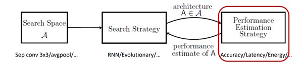
Figure 1. Overview of NAS

First, search space defines the activation function, number of layers, number of nodes, etc., that we can select. The more options there are in the space, the higher the possibility of finding the optimal architecture, which also results in more time and cost. Next, there is a search strategy for determining which to select in the defined space to find the architecture. Reinforcement learning or evolutionary methods can be used for this. And the searched architecture estimates its performance. Once the performance is measured, the results are again used to find the following architecture. Though there are many variations, such a process is the most common one. Simply, it is the method of searching and repeatedly estimating to find the optimal architecture. 

How can we reduce search costs?

As initial NAS that repeated numerous experiments required a very long time and high costs, it was inevitable to find a way to reduce cost. Since then, many methods have been researched to cut the search cost, and Table 1 summarizes the proposed methods according to the objectives.

Stabilizing Gradient-Based NAS and Training One-Shot Models	- Weights warm-up - Regularization and loss landscape smoothing - Normalization layers
Speeding up NAS	- Performance predictor - Proxy tasks - Speeding up the optimization process via sequential search - Pre-optimized search spaces
Improving the final performance	- Deriving optimal architectures from the search process - Hyperparameters, data augmentation and other tweaks for boosting Performance

Table 1. Techniques for reducing costs and improving the performance of NAS¹

The highest cost in the NAS steps involves estimating performance. This is because it is the process of inputting data in the searched architecture and learning. If the entire space is to be searched and performance is to be measured, it requires learning for all possible cases. That is why methods for predicting the performance of the searched architecture by learning just partially or none are coming to the fore. Whether it has a better architecture than others are more important than the final performance. Therefore, this can be viewed as an issue with ranking prediction.

There are 15 accepted papers related to NAS in this NeurIPS 2021. Table 2 is a table categorizing each paper by approach method. This paper will review the papers on predictors, among others, in Table 2. Reviews were conducted on what kind of predictors there are and details of its performances.

Quantization	•       Bai et al. “BatchQuant: Quantized-for-All Architecture Search with Robust Quantizer”
Meta Learning	•       Jeong et al. “Task-Adaptive Neural Network Search with Meta-Contrastive Learning” •       Lee et al. “Hardware-Adaptive Efficient Latency Prediction for NAS via Meta-Learning”
Graph Neural Network	•       Qin et al. “Graph Differentiable Architecture Search with Structure Learning”
Ensemble	•       Zaidi et al. “Neural Ensemble Search for Uncertainty Estimation and Dataset Shift”
Proxy task	•       Li et al. “Generic Neural Architecture Search via Regression”
Predictor	•       Lu et al. “TNASP: A Transformer-Based NAS Predictor with a Self-Evolution Framework”, •       Ning et al. “Evaluating Efficient Performance Estimators of Neural Architectures” •       Ru et al. “Speedy Performance Estimation for Neural Architecture Search” •       White et al. “How Powerful Are Performance Predictors in Neural Architecture Search?” •       Wu et al. “Stronger NAS with Weaker Predictors”
Others	•       Chen et al. “Searching the Search Space of Vision Transformer” •       Cui et al. “Differentiable Synthesis of Program Architectures” •       Gao et al. “Progressive Feature Interaction Search for Deep Sparse Network” •       Li et al. “Neural Architecture Dilation for Adversarial Robustness”

Table 2. Accepted papers related to NAS at NeurIPS 2021

How powerful are performance predictor in NAS¹

When NAS was first proposed, compared to learning countless neural network architectures and evaluating performance to find the final result, recent studies used an efficient strategy of predicting performance while learning just parts of it or not learning at all. Figure 2 shows several performance predictors that will be compared in this study.

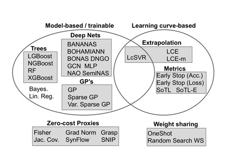
Figure 2. Types of performance predictors²

Many performance predictors are used by encoding and inputting neural network architectures while applying a method of learning models by targeting the final performance for each structure. Such an approach is popular since it is simple and easy to embody, but as the final performance is the target, there are cases in which multiple completely learned models are required to make the predictor.

Many predictors have been evaluated with limited data to make the corresponding predictor. When comparing between predictors, it isn’t easy to know which predictor has better performance. Another problem is that the experiment environment or set limitations are entirely different for simple comparison. That is why the authors tried to find answers to the two questions below:

(a) In what way can predictors with various methods be compared?

(b) Can higher prediction performance be obtained by using predictors having different methods altogether?

 

We will now look at how the answers to each question were obtained. First, to find the answer to question (a), the authors applied 31 predictors in four well-known search spaces and four datasets to see the results. The search spaces and datasets were NAS-Bench-201 with CIFAR-10, CIFAR-100, ImageNet16-120, NAS-Bench-101, DARTS with CIFAR-10, and NAS-Bench-NLP with Penn TreeBank. For a fair comparison, all combinations were tested. The ranks of neural networks extracted through the predictor were compared with the completely learned and extracted actual ranks to assess the predictor performance.

The Pearson correlation and rank correlation metric (Spearman, Kendall Tau, and sparse Kendall Tau) were used as the evaluation metrics. The architectures used in the train and test were generated uniformly in a random way, and data that modified the highest performance structure were also used in the experiment. In order to check how much each predictor accelerated the NAS process and its performance, the Bayesian optimization, and predictor-guided evolution methodologies were applied in the testing process.

We will first look at the predictors selected as the subject for comparison. Each predictor can be classified into a few categories depending on the design method. Each method has its feature, which is evaluated with init time and query time. Init time is short for initialization time, representing the initialization time of the predictor. In other words, it can be said that predictors that must learn in advance for a long time have a higher init time than predictors that do not require learning. Query time refers to the time it takes for the performance prediction process of the searched architecture. It represents the time it takes for the output of prediction performance from the time it is used by searching a specific architecture and inputting this architecture as the prediction process. The method that conducts complete learning will have a longer query time than the method that learns just partial amounts for finding the performance of architecture. Next, we will look at the methods and features of predictors and representative predictors.

Model-based predictors

Most model-based predictors learn based on supervised learning, and they are the predictors that approach regressive problems. The inputted X is the result of encoding the architecture, and it commonly uses a one-hot adjacency matrix. Target value Y is the final performance of the learned structure. Several methods are used for regression between this. Methods such as the Gaussian processes³, Boosted trees^4,5, GNNs^6,7, special encoding application^8,9, etc., are representative methods for predicting performance. Figure 3 shows the process of encoding the neural network with a specific vector and using it for predictor input. The feature of this method is that the initialization time is long, and the query time is short. The initialization time is long because the actual final performance must be known for supervised learning. On the other hand, after the predictor learns to a certain degree, prediction performance is generated according to the order of input, and therefore, the query time is short.

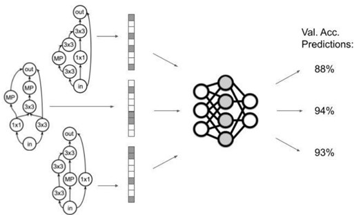
Figure 3. Use as input by encoding the neural network architecture²

Learning curve (LC) based predictors

The predictor using this method predicts performance based on a learning curve (LC). Prominent examples are applying extrapolation based on the initial learning curve^10,11 and the method of using training statistics^12,13. Figure 4 predicts future accuracy based on initial learning records using various methods. Setting the criteria allows early stopping, learning according to the predesignated threshold, or using the value that added all the losses so far. In this study, the method of adding all the learning losses is expressed as SoTL-E. This method does not require time for the predictor to learn, and it can predict performance based on initial learning records. Since it requires initial learning for each structure to predict performance, it has a long query time. 

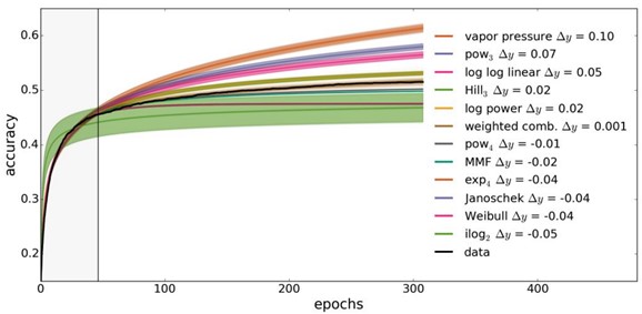
Figure 4. Final performance prediction after only completing initial learning¹²

Hybrid model-based + LC predictors

This predictor learns the predictor by adding LC and hyperparameters to the method of encoding structures. It includes primary and secondary derivative variables and deals with LC as features. Although its performance is not poor as it deals with a lot of information, its weakness is its long init time and long query time due to LC. Compared with the figure of the model-based predictor, this method can be understood as a method of encoding LC together with the structure, as shown in Figure 5. Representative predictors are the SVR¹⁴ that made and applied derivative features and Bayesian NN ¹¹ that uses the entire LC as features.

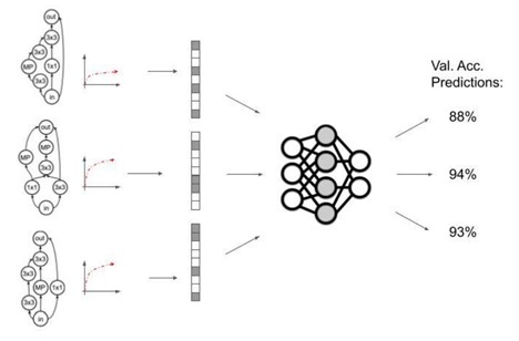
Figure 5. The hybrid model used together with LC²

Zero-shot predictor

This is a method of predicting the final performance by calculating the structure’s statistical information within 3–5 seconds. It has a very short init tie and query time, and thus, it is a method that is being frequently studied as of late. As can be known from its name, a zero-shot predictor predicts performance without learning the predictor or learning the searched neural network. This method maximizes the utilization of neural network information on input data. There are methods such as Jacobian Covariance (Jacob. Cov.)¹⁵ that uses the differences of neural network gradients for input data, and relu_logdet¹⁵ uses the state in which input is activated in each node. Figure 6 illustrates using ReLu for each node in relu_logdet to utilize the activated state as a binary code. Activated fields are encoded as one and deactivated fields as zero to use this information.

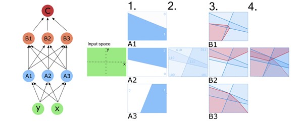
Figure 6. Visualization of ReLU-based binary activation¹⁵

Furthermore, the method is proposed by getting a hint from pruning to remove unimportant parts from the neural network architecture. This method utilizes the sensitivity of parameters in the neural network performance evaluation using a mini-batch. Synaptic Flow¹⁶ and SNIP¹⁷ fall under this method.

Weight sharing

Lastly, there is the method of making all possible items of search space in advance (super-network) and selecting some cases to search the structure while sharing the weight of the supernetwork for each structure. Predictors falling under this are One-shot¹⁸ and Random WS¹⁹. It has a short query time like ENAS²⁰ famous for weight sharing, but it has an average init time since it is necessary to compose the supernetwork early on and has to learn partial amounts. Figure 7 is an example of a super-network that shows all selectable items set in advance and selects its parts.

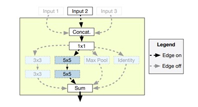
Figure 7. One-shot model evaluation¹⁸

Figure 8 is the result of measuring the performance of target predictors based on NAS-Bench-201 on CIFAR-10. The lower the init time and query time and the higher the Kendall Tau, the better the predictor. But as evident in the results, since more information can be used when learning about the predictor or architecture, higher Tau values are generally shown. Despite this, some zero-shot predictors have short times for both, but it appears to have decent performance. In particular, when considering trade-offs, Jacob. Cov. is the recommended method.

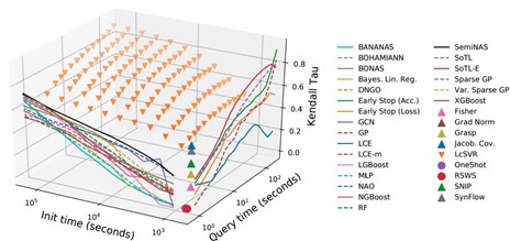
Figure 8. Performance of predictors

Figure 9 shows the best method in the corresponding block when seeing each query time and init time discretely. The left side of Figure 9 displays the results in NAS-Bench-201 on CIFAR-10. When query time is between 100 and 1,000 seconds, SoTL-E method exhibited the highest Tau throughout all init times. For lower query time and init time, the blue Jacob. Cov. method was found to be the best method. The right side of Figure 9 shows the results for other search spaces, and it is evident that the modes of results for each search space are different. When summing up the results, although SoTL-E method is the common one, note that it is relative according to the space.

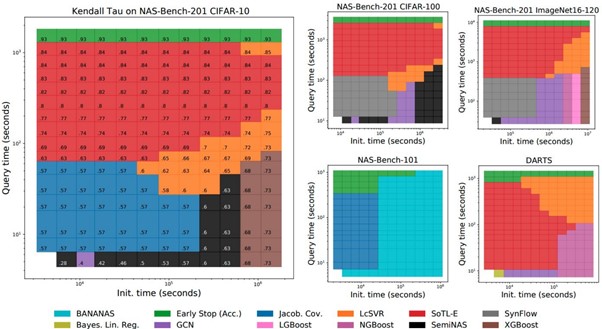
Figure 9. Predictor distribution showing highest Kendall Tau for each search space

Figure 10 is similar to Figure 9, but the values that act as the criteria for each region are not Tau, but the results of Pearson correlation and Spearman rank correlation between the prediction ranks and actual ranks. Similar to the above Kendall Tau, it was found that SoTL-E and Jacob. Cov. accounted for a significant portion.

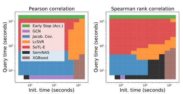
Figure 10. Pearson correlation and Spearman rank correlation of predictors

Next is an experiment on the second question to examine whether there would be a better performance by using predictors together. Among the methods that displayed good performance, the authors proposed the OMNI. This model combined the results of the LC method and zero-cost method, SoTL-E, and Jacobian Covariance, respectively, as additional features of model-based predictors. The OMNI generally showed the best predictive performance compared to single predictors, and it had certain superiority with a massive difference with the second-best predictor. This can be seen in Figure 11—the brighter the color, the more significant the performance difference.

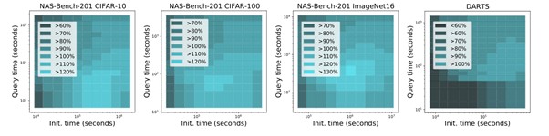
Figure 11. Kendall Tau of the OMNI compared to the second-best ranked predictor

To make a general summary, there is no short answer to how strong each predictor is. Methods of displaying outstanding performance differed depending on the init time and query time region, along with search space and dataset. Figure 12 shows the average results for all search spaces used in the experiment. SoTL-E and Jacob. Cov. fields are found to be generally broad for all experiments. And mixing predictors with various methods showed as much as 120% or higher prediction performance than using a single predictor.

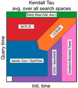
Figure 12. Kendall Tau average for all search spaces

Conclusion

This paper examined performance predictors of NAS through reviews on accepted papers at NeurIPS 2021. There is plenty of room for improvements for various methods other than predictors; this is a field where many studies can be conducted. However, there are some points to watch out for in applying existing studies. Since it is tough to maintain performance while conserving time and resources, extra precaution regarding the trade-off relationship is needed. It is necessary to decide in advance which direction to go for. And while NAS generally exhibits satisfactory performance, the limitations are that an environment equipped with some degree of infrastructure is needed and that research focusing on image and natural language processing is still underway. In particular, there are relatively few studies applied to time-series. As time-series data has relatively less information than images, it is more sensitive to search space and search strategy. That is why it is challenging to find NAS methodologies that can be robustly applied. But if this puzzle can be solved, it will be possible to create an appropriate prediction model without designing the neural network considering every aspect for various time-series. As relevant studies are being conducted rapidly, it can be anticipated that the solution will be found sooner or later.