[ICLR 2022] Part 2: Time Series Anomaly Detection

This year marks the 10th anniversary of the International Conference on Learning Representations (ICLR), the most prominent conference in the world in the field of deep learning that was first held in 2013. It is also a venue for the dissemination of cutting-edge research and publications in all fields that employ deep learning, including artificial intelligence, data science, vision, speech recognition, and robotics. We introduce some of the papers presented by LG AI Research at the online ICLR 2022 conference held in April. - Part 1: Efficient Transformer — Junghee Kim, Applied AI Research Lab - Part 2: Time Series Anomaly Detection — Yeseul Shim, Applied AI Research Lab - Part 3: Reinforcement Learning as a sequence modeling problem — Deunsol Yoon, Applied AI Research Lab

Introduction

Anomaly detection refers to the task of detecting anomalies that are judged to be different from the existing measurements as it does not follow normal patterns within the data. This can be used in various domains, namely risk management, video security and fraud detection.

Traditional methods of anomaly detection include One-Class Support Vector Machine^[1] and Kernal Density Estimation^[2]. Such traditional methods have limitations in completely learning the diverse and wide-ranged dynamics of time series data and in generalizing the unseen real-world scenario. In particular, it has already been confirmed in many studies that performance falls for high-dimensional data collected through the recent development of various sensors, equipment, etc.

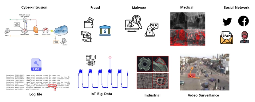
Figure 1. Major Cases of Anomaly Detection^[3]

In order to overcome the limitations of the performance of the traditional anomaly detection method, studies on applying deep learning models to complex time series data including high-dimensional data (e.g. image, voice) have been conducted and made many achievements. This blog introduces the basic concept and method of approach to time series anomaly detection issues based on deep learning, and introduces two theses related to time series anomaly detection published recently at the ICLR 2022.

Deep Learning-Based Anomaly Detection

Systems such as industrial equipment and space probes monitor and collect data using numerous sensors. System data is continuously measured, and various forms of time series data are collected in real-time. For this, time series anomaly detection must be able to learn major informative representation in such complex and various large-scale data dynamics. Creating decision boundaries to detect and easily distinguish highly rare anomalies in numerous normal data is also important.

If normal and abnormal labeling is sufficient in training data, the supervised learning method that uses all the labeled information to judge anomalies for test sets can be applied. However, labeling for anomalies does not exist in real world data, and most of the time, it is impossible to define the anomaly. Therefore, in the case of the supervised learning approach, when unseen anomaly test data comes in as input into the model, it has the weakness that it cannot respond to anomaly judgments. On the other hand, unsupervised learning-based anomaly detection can learn with just normal data, and thus does not require additional work such as detailed labeling for anomalies. Furthermore, it can also respond to completely new anomalies that do not exist in data.

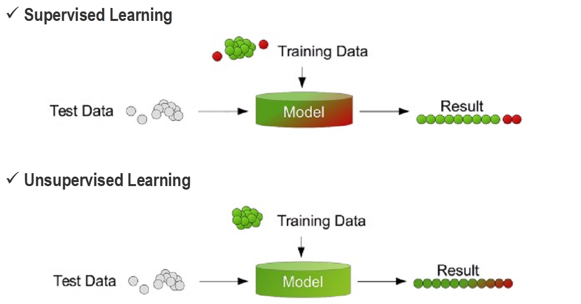
Figure 2. Supervised Learning and Unsupervised Learning^[4]

Therefore, due to the situations and conditions of data in the real world, research is being conducted mainly on deep learning-based unsupervised anomaly detection. The basic concept of the unsupervised anomaly detection model can be seen in Figure 3. Such a method trains the reconstruction model, such as Auto-Encoder, with just normal data to create a model that can reconstruct normal data well. Through this, deep learning model can precisely reconstruct complex normal data.

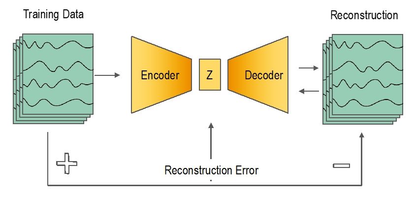
Figure 3. Auto-Encoder-Based Anomaly Detection Model Learning

Once the reconstruction model based on Auto-Encoder is trained properly, the model can reconstruct data to a normal state to a degree similar to normal data input. In this case, there is small error between input and output. On the other hand, for the new data input that the model has never seen before, as the model only knows normal data, it is still reconstructed into normal data. In this case, the error between input and output (reconstruction value) becomes large. The model can detect anomaly based on this reconstruction error.

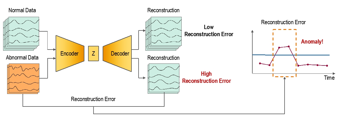
Figure 4. Auto-Encoder-Based Anomaly Detection Model Inference

Based on such a basic concept, the industry is actively conducting research on anomaly detection based on various model structures such as simple Auto-Encoder structures to Variational Auto-Encoder, GAN structure, and Adversarial Auto-Encoder^[5,6,7]. Particularly in the case of time series, models using RNN and ConvLSTM structure are being proposed to properly reflect time series data information.

However, these simple deep learning models also have a few limitations. The model’s learning abilities for data reconstruction are too effective that it often reconstructs even abnormal data. In addition, when utilizing structures such as LSTM, information on hidden representation can actually be lost. If numerous normal data already exist in this case, it can cause abnormal data to be buried. The model judges anomalies by calculating the reconstruction error in each time step. As it is computed as points, it cannot reflect the temporal context of time series.

We will introduce two studies on time series data among multiple papers on resolving the anomaly detection issue submitted at ICLR 2022. Both studies proposed appropriate model structures and methodologies for time series data, thus being able to secure high performance in time series data anomaly detection targeting benchmark datasets.

Anomaly Transformer

The first study is titled Anomaly Transformer: Time Series Anomaly Detection with Association Discrepancy^[8]. As evident in the title, this study proposes an anomaly detection method using the transformer. Transformer is a deep learning model structure that brought huge development in the NLP sector since being announced by Google in 2017. This study proposed a structure for changing the existing transformer structure to be appropriate for anomaly detection, and to be used as an anomaly transformer. In order to understand the idea suggested in this study, the following three terms defined and presented by the author must be understood.

- Series Association: Temporal context information association of overall time series data at each time point
- Prior Association: Adjacent-concentration association of time series data
- Association Discrepancy: Difference between prior-association and series association at each time point

This study proposes the terms of prior association and series association, and extracts these two values from the time series data and uses the difference between the two values as the criterion of anomalies. Furthermore, it proposes a few inductive bias ideas for the anomaly detection as follows.

- As abnormal values are rare, they do not have a strong association with general time series, but exhibit different tendencies.
- Normal data exhibit informative association for not only adjacent areas, but for the entire time series.
- Due to the continuity feature of time series, abnormal values are concentrated in adjacent areas.
- Such characteristics of abnormal value are shown as association discrepancy.

The model structure and idea proposed in this study are as shown in Figure 5, which can be largely divided into three blocks: prior association extraction, series association extraction, and minmax strategy. The prior association represents adjacent information/prior in the time series data as defined earlier. This prior association extracts association between adjacent data at each data point.

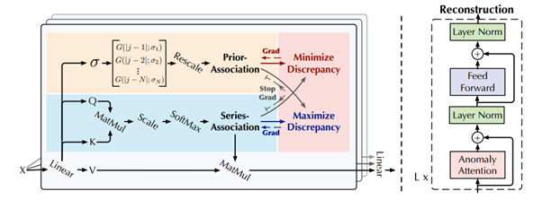
Figure 5. Anomaly Transformer Model Structure

The process for extracting prior association is as follows. First, prior is calculated for relative temporal distance using the Gaussian kernel. Here, the learnable scale parameter $\sigma$ can be applied to various time series patterns to calculate prior association.

Series association is used to calculate the overall association of data over a longer time than the prior association. In this study, the attention value and the estimation process in the existing transformer model were used as-is for extracting series association. When expressing the calculation of the said prior association and series association as an equation, it is as follows.

 

This study proposed a concept called association discrepancy that represents the difference between prior association and series association based on these two association values. There are many ways to calculate the difference between these two distributions, but in this study, the difference between the two distributions was calculated with the Kullback-Leibler divergence value. The main idea of this is that the association discrepancy can be used for judging normal/abnormal. Through this, it is possible to calculate prior association and series association by each layer, and the average value of L number of layers was calculated with association discrepancy. The equation for calculating association discrepancy can be expressed as follows. S and P stand for series association and prior association, respectively.

According to inductive bias proposed in this study, prior association reflecting adjacent distribution at the time of anomaly and the total series association have the same distribution that is given attention, and therefore, association discrepancy is found to be small. Meanwhile, in the case of normal data, since the part that the series association of the entire time series data pays attention to is not near normal data, the association discrepancy is found to be large.

The association discrepancy deduced as such was used as a loss function for training the anomaly transformer model. In this case, as it learns as an unsupervised task assuming it to be a situation with no label for anomalies, both reconstruction error and association discrepancy are used as a loss. As the model is being trained, reconstruction error is minimized and association discrepancy is maximized. In other words, the model learns so that there is a high reconstructive ability for normal data used in learning and to make the distribution difference between prior association and series association high.

Moreover, reconstruction error and association discrepancy were both used in the anomaly score that judges the level of anomaly in this study. In the case of normality, reconstruction error is small and association discrepancy is large. In the case of anomaly, reconstruction error is large and association discrepancy is small, thus giving it a high anomaly score. At times, reconstruction works well unlike intended in anomaly data, thereby causing reconstruction error to be shown as being small. But even in this case, as the association discrepancy is still small, it is possible to detect anomaly cases well. Anomaly score can be expressed as an equation as follows.

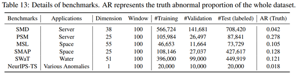
In order to verify the performance of the anomaly transformer structure, this study used the following six datasets. The datasets in the table below are widely used when verifying time series anomaly detection models. It is composed of anomaly situations in servers, anomaly situations of satellites revealed by NASA, and Time Series Benchmark dataset^[9] introduced at NeurIPS 2021. Dimension represents the number of features of time series data, and AR represents the ratio of actual anomalies distributed within the dataset to verify actual performance.

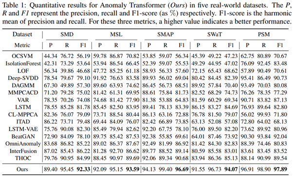
Performance comparisons of anomaly transformers with existing anomaly detection studies such as OCSVM and Isolation Forest can be checked in the table below. Anomaly transformer showed the best performance among all the datasets based on F1 score.

When visualizing the actual NeurlPS-TS data standard detection results, it was found that the anomaly transformer could detect abnormal data that could not be detected by other models. The first row shows time series data for verification including actual abnormal patterns, and the row below shows the detection results in the order of BeatGAN, Deep-SVDD, LSTM-VAE, and Anomaly Transformer. When there is a high anomaly score for anomaly sectors, it can be viewed that anomalies are detected properly. The graphs indicated with red boxes in Figure 6 are cases that were not detected. It is evident that there was no big score difference for normal and abnormal sectors, and that it failed to detect anomalies. However, in the case of anomaly transformer, as anomaly score rose in the anomaly point, it was able to accurately detect anomaly points.

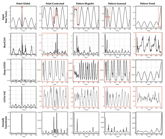
Figure 6. NeurlPS-TS-Based Actual Anomaly Detection Case

To summarize the anomaly transformer study, it proposed a new anomaly standard called association discrepancy and suggested an anomaly detection model structure using time series self-attention based on transformer structure. This study configured simple inductive bias as a model and demonstrated improved performance in various time series benchmark datasets. However, there are still insufficient theoretical explanations and evidence for the model proposed in the study.

Graph Augmented Normalizing Flow

The second study is GRAPH-AUGMENTED NORMALIZING FLOWS FOR ANOMALY DETECTION OF MULTIPLE TIME SERIES^[10]. As can be known from the title, this study is an attempt at anomaly detection in time series data using graph structure and normalizing flow. We will explain the concept of normalizing flow utilized in this study in an easy-to-understand manner.

Normalizing flow is a method presented to predict complicated probability distributions. Normalizing flow applies a series of inverse functions from a simple probability distribution (usually Gaussian distribution) to gradually convert to a complicated probability distribution. Through this series of conversion and change-of-variables theorem, we can repeatedly replace new variables from simple distributions and ultimately obtain the probability distribution of the targeted final variable. The advantage of normalizing flow is that unlike GAN or VAE, the likelihood of input data for models can be calculated directly. In other words, it means that explicit and tractable models can be developed.

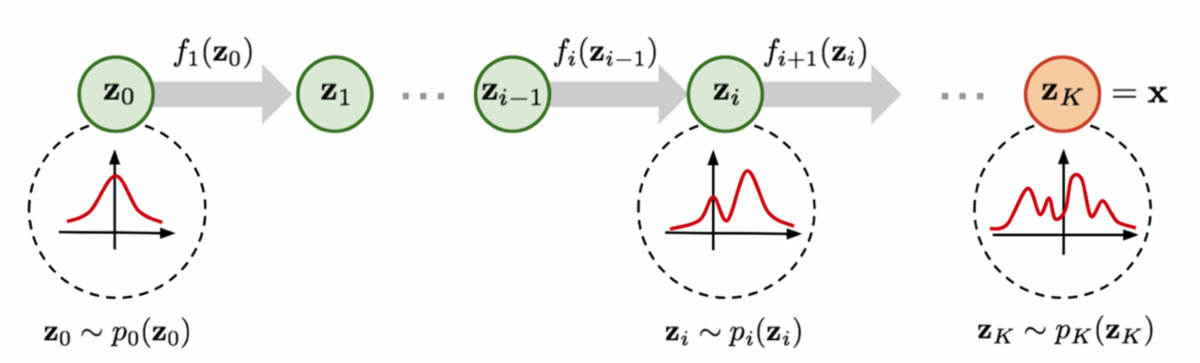
Figure 7. Normalizing Flow Concept^[11]

This study utilized normalizing flow where multivariate time series data are converted into a graph format. In multivariate time series, by considering each input as a single node, it can be expressed as a Bayesian network. The joint distribution of Bayesian network for N number of variables can be expressed as shown in the following equation. Here, $X^i$ represents multivariate time series and $pa\left(X^i\right)=\left\{X^i:A_{ij}\ne 0\right\}$ represents the parents set of $X^i$. At each time point t, the density of $X_t^i$ is affected not only by the graph parents, but also by prior history, $X_{1:t-1}^i$, and is expressed with the equation below. 

As all the data lengths are different, conditional information $pa\left(X^i\right)$ and $X_{1:t-1}^i$ cannot be used right away with parameterization. However, in this study, it can be shortened to vector $d_t^i$ having a certain length of conditional information through the dependency encoder model based on the proposed graph. At this time, conditional normalizing flow $p\left(X_t^i\overline{)pa{\left(X^i\right)}_{1:t},X_{1:t-1}^i}\right)$ is the same as $p\left(X_t^i\overline{)d_t^i}\right)$.

The general model structure proposed in this study is shown in Figure 8 below. Input data is transformed based on the aforementioned Bayesian network and the adjacency matrix is calculated for use as graph convolution layer input. In the case of original time series data, RNN structure suitable for time series data is used to extract hidden state H. The extracted hidden state H is used as input for the graph convolution layer, and the integrated dependency representation $Dt=\left(d_t^1,\cdots ,d_t^n\right)$ value is calculated. The overall Dependency Encoder structure uses both this graph convolution and RNN. The equation for extracting hidden state $h_t^i$ and dependency representation $D_t$ at each time point from the time series data is as follows.

Using the representation $d_t^i$ extracted through the dependency encoder, normalizing flow can be used to calculate the conditional density of $x_t^i$. The log density equation can be finally calculated for multiple time series X based on this equation. The equation for calculating conditional density and log density are as follows.

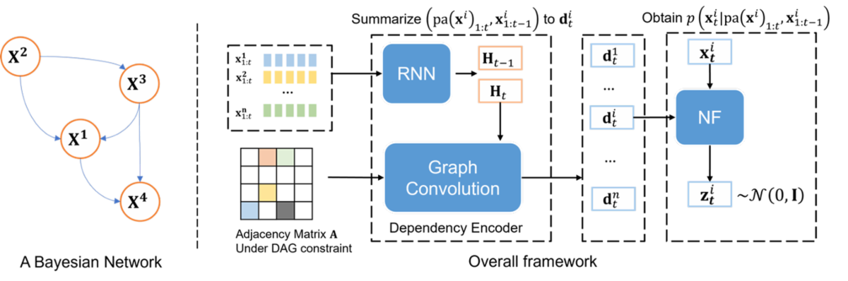
Figure 8. Graph Augmented Normalizing Flow (GANF) Structure

According to the general training of normalizing flow, the objective function used the joint density of the training data. This is the same as the Kullback-Leibler divergence between distribution with real data and distribution which computed by flow. When expressing this as an equation with regularizations for the adjacency matrix, it is as follows.

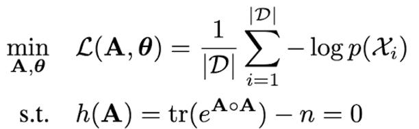
After training the model, the anomaly score that acts as the standard for judging normality and anomaly is based on the input multivariate time series’ log density ($log\left(p\left(X\right)\right)$). As anomalies are rare compared to normal data, it is assumed that density is low.

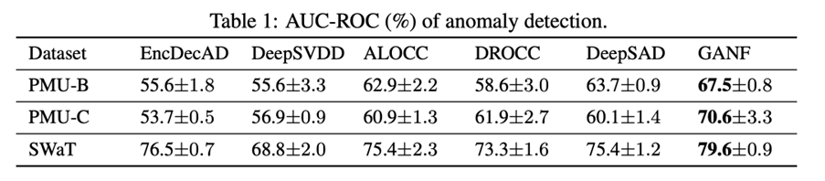
PMU-B, PMU-C, and SWaT datasets were used to verify the performance of the model proposed in this study. PMU-B and PMU-C are Phasor Measurement Unit data collected for a year by the Smart Grid of the U.S. These are data that domain experts labeled intermittently occurring events as anomalies. They are not open data, but verified datasets used by the author for research. The author also conducted verification in the open data, SWaT. Furthermore, in order to compare the proposed model structure, performance between datasets corresponding to deep learning-type models researched in the past was compared. AUC-ROC was used as the standard for comparing performance, and the bigger the AUC-ROC, it was judged to a model with better performance. As shown in the table below, Graph Augmented Normalizing Flow (GANF) proposed by the author had the best performance for the three datasets compared to the remaining five baseline models.

When examining the actual AUC-ROC graphs, it is as follows. The green line in the graph below shows the performance of GANF. It showed the best performance for all three datasets of PMU-B, PMU-C, and SWaT.

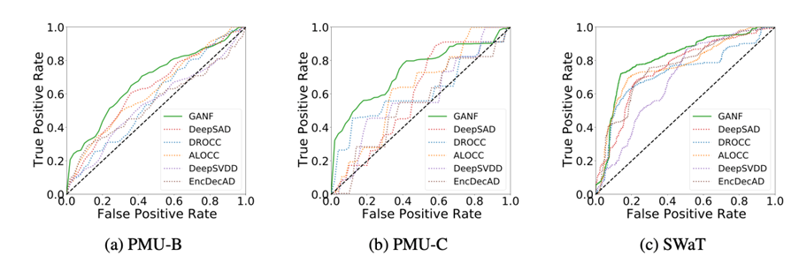
Figure 9. ROC Curve of Anomaly Detection Model Targeting Datasets

The performance of models for the actual time series data anomaly detection can be checked in the graph below. As GANF model measures anomaly based on low density, a density that serves as the criteria for anomaly at the time of anomaly is shown to be small. In the figure below, the time of anomaly is indicated with a red line. It is evident that the anomaly score of the blue graph at the time of anomaly dropped.

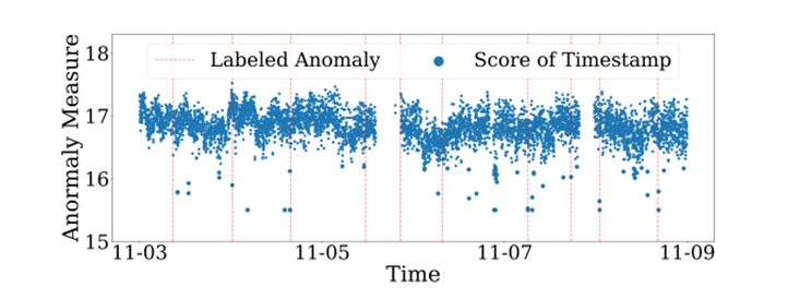
Figure 10. Anomaly Detection Results in Actual Time Series Data

To summarize the GANF study, multivariate time series data were transformed into input format based on the graph and the normalizing flow was used to learn the density of the input data for calculation as a model that judges anomalies. While it is significant in that the model was verified using datasets actually in operation, performance in the benchmark dataset is calculated for only one set, and therefore, additional verification for performance is required. For sensor data or specific data with a high association between time series data, it is judged that GANF proposed in this study would be meaningful.

Conclusion

We introduced researches related to anomaly detection for time series data presented at the ICLR 2022. In the real world, anomaly detection has to be approached based on unsupervised learning due to the lack of labeling. Therefore, in the initial stages of deep learning anomaly detection, anomalies were extracted with reconstruction error or distance in the embedding space.

The two studies introduced today trained the model according to the data situation with some inductive bias for data or problem cases, and the anomaly score was designed as the criteria for anomaly detection according to the model structure. By developing upon the methodologies proposed in each study and studying models and methodologies based on an inductive bias that can be understood and applied in any situation, it will become possible to secure ideal anomaly detection technologies for time series data.