[ICLR 2021] Part 1: Neural Combinatorial Optimization in ICML 2021

The International Conference on Machine Learning 2021 (ICML 2021) is a large-scale international conference that attracts around 70,000 participants each year. This year marks the 38th iteration. It is also one of the most influential conferences in the field of artificial intelligence with thesis acceptance rate of 20% and impact factor of 6.99. Here is a summary of the meaningful research papers shared at the conference, picked by three researchers from LG AI Research who participated in the ICML 2021 held online from July 18 to 24. - Part 1: Neural Combinatorial Optimization in ICML 2021 - Kanghoon Lee from Di Lab - Part 2: Generative Models for OOD Detection in the ICML 2021 - Hyemin Jung from Di Lab - Part 3: Spatio-temporal Time-series Forecasting in ICML 2021 - Juhyun Lyu from Di Lab

The Data Intelligence Lab of the LG AI Research has the goal of finding meaningful information from various types of data encountered in real life and identifying and solving problems that have not been solved so far through this. There is Combinatorial Optimization^[1], a problem that has not received much attention in the latest artificial intelligence and machine learning methodologies represented by Deep Learning, although it is very common and easily encountered in reality especially in the industry.

Represented by the Traveling Salesman Problem, Minimum Spanning Tree, and Knapsack Problem, Combinational Optimization is a field of mathematical optimization that refers to issues that students majoring in computer science may have heard of at least once in an algorithmic class. As a characteristic of Combinatorial Optimization problems, the area of the feasible solution must be discrete or discretely reduceable. Many of these problems are difficult problems belonging to NP-Complete[2] in the Computational Complexity Theory but remain unresolved; they have recently been recognized as a very challenging problem for AI researchers.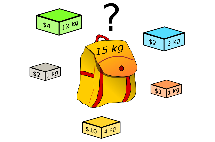

Figure 1. Example of knapsack problem^[3] 

 
The Knapsack Problem in Figure 1 shown above is a problem of choosing a combination of items that maximizes the sum of values within the range of not exceeding the maximum knapsack weight of 15 kg, when there is a knapsack that can hold up to 15kg and there are items each of which has specific value and weight. This Knapsack Problem is a problem that can be easily encountered in real life, such as when choosing clothes to put into a suitcase and luggage or when trying to load cargo considering the maximum load weight in cargo transportation. In Figure 1, the Optimal Solution is to choose the remaining four items (Grey: $2, 1kg, Yellow: $10, 4kg, Red: $1, 1kg, Blue: $2, 2kg) except for the light green item that has a value of $4 but is too heavy at 12kg. The four items selected in this way have a total weight of 8 kg, which meets the condition of the maximum weight of the backpack being 15 kg or less but has total value of $15, the highest value of any possible combination of items considered under the constraint of maximum weight of 15 kg.

The representative features that can be observed in the Knapsack Problem above are: (1) whether each item is selected or not can be expressed as a binary variable “0-1,” and (2) the total number of combinations of choices that can be thought of from 5 items is 32 (= 2⁵) in a discrete environment. In particular, what we should look at closely from the second characteristic is the fact that as the number of items increases, the combination of choices we have to consider becomes 2^{number of items}, which increases exponentially. As such, even if the size of the problem increases linearly, the phenomenon of the area of feasible solution to be considered to solve the problem growing exponentially appears in many combinatorial optimization problems; this phenomenon can be said to be the biggest characteristic and difficulty of combinatorial optimization problems.

The mathematically generalized definition of the knapsack problem is as follows^[3]: There are n items {x₁, x₂, ... x_n}, and each item x_i ∈ {0,1} (however,  i ∈ {1,2, ..., n}) is a binary variable, so you can express that you choose item x_i and put it in the knapsack x_{i = 1} or do not choose item x_i and do not put it in the knapsack x_{i = 0}. Moreover, assuming that the maximum weight of the items that the knapsack can hold is W ∈ R⁺ and each object x_i has value of v_i ∈ R⁺ and weight of w_i ∈ R⁺, the knapsack problem can be expressed by integer programming (Integer Programming or Integer Linear Programming) as follows:



At this time, the total number of items n, the value and weight of each item, and the maximum weight W of the knapsack are given from the definition of the problem; , which indicates whether or not to choose the items to be put in the knapsack, becomes the variable to be determined through the integer programming above. In integer programming, the variable is a set of integers belonging to a discrete environment, and the objective function (i.e., ) and constraints (i.e., ) that need to be optimized are expressed as linear functions, so it is called Integer Programming or Integer Linear Programming, etc. In integer programming, the optimization objective functions and constraints are still linear functions; when the set of variables is a set of continuous real numbers, it is called Linear Programming.

Linear programming is generally known to be able to calculate an optimal solution efficiently through the Simplex Method, etc.. In the case of integer programming, the values that variable can have are discrete, and the number of all possible cases is 2ⁿ; this means that as the number of variables n increases, it increases exponentially, so calculating an efficient optimal solution is known to be very difficult. In addition, when the variable is a mixture of integers and real numbers, it is called Mixed-Integer Programming or Mixed-Integer Linear Programming; calculating an efficient optimal solution like integer programming is generally known to be very difficult.

If the problem is defined by integer programming like the knapsack problem above, you can find an optimal solution to the problem by using a mathematical optimization software package. A representative software package for mathematical optimization is CPLEX^[4]. CPLEX is the most representative mathematical optimization tool in linear programming, providing optimization functions in integer programming and mixed-integer programming as well. Optimization tools mainly used recently in integer programming problems (or mixed-integer programming) are GUROBI^[5] and SCIP^[6]; while GUROBI can be used for a fee, SCIP has the advantage of being free to use. You can also perform the mathematical optimization above through Google's OR-Tools^[7].

If you use a mathematical optimization software package, it is basically easy to describe a combinatorial optimization problem and find an optimal solution, but there is a limit, i.e., even if the complexity (number of variables and constraints) of the problem to be solved increases only slightly, the quality of the optimal solution obtained by the software package drops sharply. In order to overcome this limit, the field of Neural Combinatorial Optimization studies combinatorial optimization through data-based learning using deep learning, and it has recently attracted a lot of attention. Representatively, there was a study titled "Pointer Networks"^[8] that tried to solve combinatorial optimization problems with Supervised Learning in 2015, including a study titled "Neural Combinatorial Optimization with Reinforcement Learning^[9]," which introduced the method of Deep Reinforcement Learning in 2017. In the recent study "Neural Branching + Neural Diving^[10]: proposed by researchers in Google and DeepMind, the performance and scalability of mixed-integer programming have been greatly increased by combining Tree Search and Deep Learning and mathematical optimization software package SCIP^[6].

A number of meaningful deep learning-based combinatorial optimization study results were announced at this year's ICML 2021. In particular, there have been many attempts to solve various combinatorial optimization problems encountered in the real world through an appropriate combination of the existing mathematical optimization-based integer programming and the latest data-based deep learning methodology; among these, two research results, (1) Neural A* Search^[11] and (2) CombOptNet^[12], are introduced below.  


Path Planning using Neural A* Search (Yonetani et al., ICML 2021) 

Path planning is the problem of finding the optimum path from a given starting point to a destination. Path planning, such as navigating a driving path to a destination using a car, is very closely related to our daily life, and many people make calculations based on the path they know in their head or use a map app on their smart phone to find and use the shortest path. A* Search^[13] is a representative path planning algorithm, and it uses an appropriate heuristic function to increase the efficiency of the search while maintaining search accuracy. Thus, it is used as a basic algorithm for path search in many navigation systems.

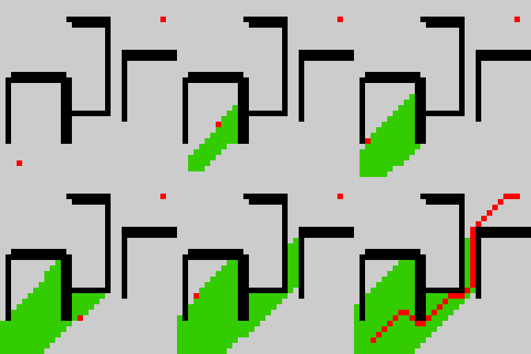Figure 2. Example of A* path search^[14] 

  
Figure 2 is an example of an A* path search algorithm. As shown in the figure, the problem involves finding the shortest path starting from the red dot on the lower left to the red dot on the upper right, and the red dot on the lower left cannot pass the wall of the black area. At this time, the A* path search algorithm sequentially searches the surrounding areas marked with green on the figure to move toward the destination, the red dot on the upper right. When the A* algorithm reaches the red dot on the upper right corner, the green area representing the search history represents the time or cost spent searching for a path, and the final path obtained after paying for this search is expressed by a red line.

Figure 3. Example of image-based path search^[14] 

 
This study proposes Neural A* Search, which includes data-based learning for the A* search algorithm to work not only in the synthetically created problem like the path search example in Figure 2 but also in the prediction of the path of pedestrians in the image-based real photo as shown in Figure 3.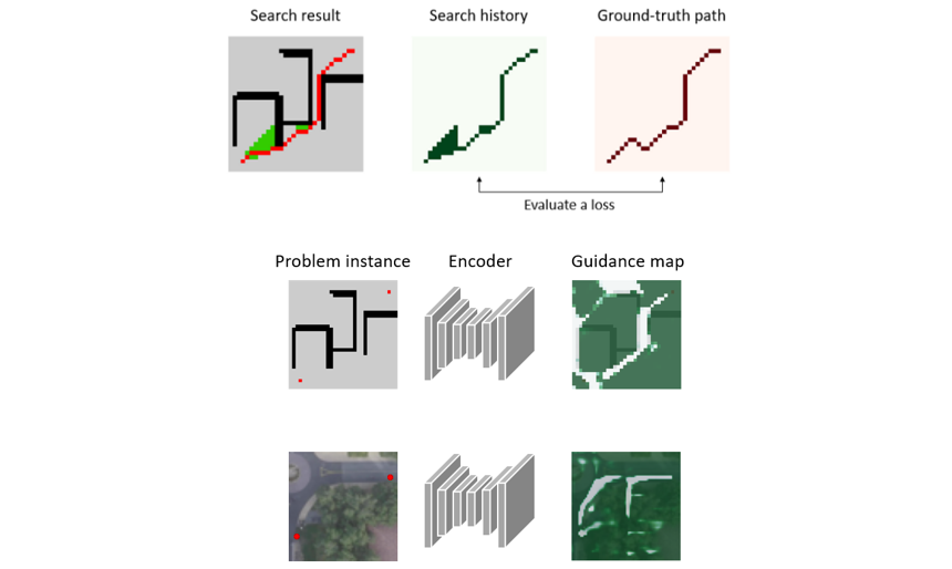

Figure 4. Data-based Guidance Map learning and transformation^[14] 

 
The Neural A* algorithm can increase the efficiency of search compared to the existing A* algorithm thanks to the Guidance Map, which provides information on the paths of candidates with high priority when searching for a path from a given Problem Instance. As shown in Figure 4, the Guidance Map is learned in a direction that minimizes the difference between the green area, the history that the A* algorithm has searched for to find the optimal path, and the Ground-Truth Path. The obtained Guidance Map serves as a heuristic function required by the A* algorithm, so the efficiency of search of the Neural A* algorithm increases as the Guidance Map provides information closer to the actual correct path.

Figure 5. Neural A* algorithm schematic diagram^[11]

 
Figure 5 shows the overall process of the Neural A* algorithm. As explained earlier, if a problem example is given, a Guidance Map can be obtained from the trained Encoder network. The obtained Guidance Map serves as a heuristic function of the A* algorithm; in the second stage of Neural A*, efficient A* tree search is performed using the heuristic function obtained like this. Finally, the search history data resulting from the A* tree search is used to re-learn the Encoder network for the Guidance Map in the direction of reducing the difference from the actual correct answer path.

Here, as the most important contribution of this study, the Differentiable A* Module can be seen. In general, A* search is done in a discrete environment, which means that the gradient does not flow in the second stage in Figure 5; thus making it impossible to update the Encoder network. To solve the problem above, the authors devised a method of replacing the operations required in the existing A* algorithm with a matrix-based operation, which enabled implementing a differentiable A* module.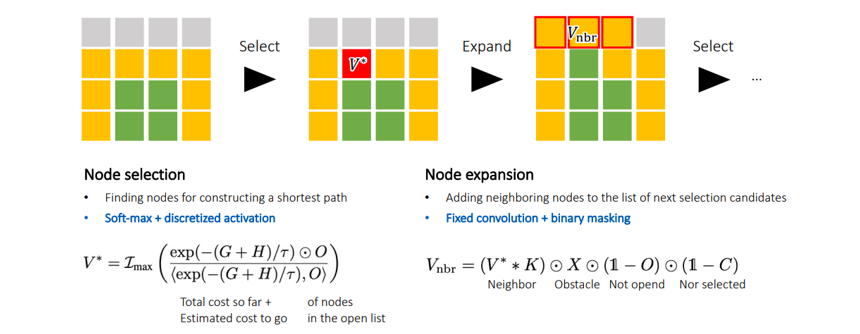

Figure 6. Matrix-based differentiable A* tree construction^[15]

Figure 6 shows the Tree Construction in the Neural A* algorithm. The A* algorithm creates a search tree through construction, and the nodes that have actually been searched are managed under the name of green closed list; candidate nodes adjacent to the closed list to be searched are managed under the name of yellow open list. An efficient A* search tree selects the red node with the highest heuristic-based value (calculated from Guidance Map, etc.) among the nodes in the yellow open list, and the selected red node is now moved to the closed list and the tree is constructed by adding new nodes adjacent to the red node to the open list. The entire process generally requires discrete operations, but in Figure 6, the closed list and the open list are expressed as binary matrices C, O indicating whether each node belongs to each list; each binary and the matrix V*, which represents the values of the matrices and nodes, etc., are updated using the convolution operator ⊙.

Going back to Figure 5, we can see that the intermediate module wherein the A* tree search is performed is replaced with matrix-based differentiable operations as shown in Figure 6, and it has a structure that allows the gradient to flow up to the Encoder network to get the Guidance Map from the Loss function for the difference between the search history and the actual correct answer path.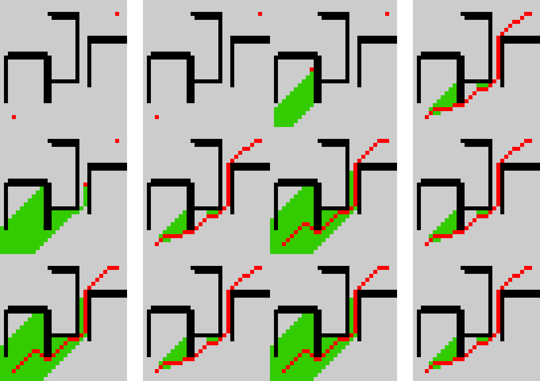

Figure 7. Comparison example of existing A* path search (left) and neural A* path search (right)^[14]

 
Figure 7 shows a comparison between the path searched by the general A* algorithm on the left and the path searched by the Neural A* algorithm through Guidance Map learning on the right. It can be seen that the Neural A* algorithm has much less green area indicating the time required for path search, suggesting that it finds the optimal path faster.

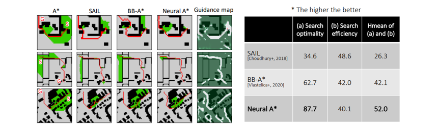
Figure 8. Point-to-Point optimal path search comparison experiment^[15]

Figure 8 compares the Neural A* algorithm with the existing optimal path search algorithm through data-based learning. It can be seen that the Neural A* algorithm has much less green area indicating the efficiency of the search, and that the generated path is also closer to the shortest path.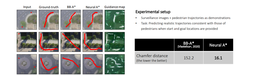

Figure 9. Optimal path search comparison experiment in the actual image^[15]

Figure 9 shows the experimental results of the movement path in the actual road image. As shown in Figure 8, the result of the Neural A* algorithm has been learned to be closer to the correct answer path.

So far, we could see that it is possible to search the more efficient learning-based optimal path by using Guidance Map and differentiable A* module through data-based learning for A* search, a representative path planning algorithm. The fact that data-based learning was possible by differentially constructing the A* search, which was previously defined in a discrete environment, was the most important aspect to be examined in this study. In the heuristic-based tree search algorithm like the A* algorithm, however, the level and search efficiency of the obtained path are determined depending on which heuristic function is used, and it was a little disappointing that there were experimental results but no mention of the case before the meaningful Guidance Map was learned or when the learning of the Guidance Map failed. In addition, one of the great advantages of A* search is that it is possible to provide theoretical guarantees for optimal path search for admissible heuristic functions, but one of the regrets was that such theoretical guarantees were omitted by using the learned Guidance Map immediately as a heuristic function in Neural A* search.

* Reference Paper http://proceedings.mlr.press/v139/yonetani21a/yonetani21a.pdf Slide https://icml.cc/media/icml-2021/Slides/9055.pdf Video https://crossminds.ai/video/path-planning-using-neural-a-search-614bd1e23c7a224a90903035/ Blog https://omron-sinicx.github.io/neural-astar/ Source code https://github.com/omron-sinicx/neural-astar

CombOptNet: Fit the Right NP-Hard Problem by Learning Integer Programming Constraints (Paulus et al., ICML 2021)

In the integer programming that we looked at earlier in the knapsack problem, the variable to be determined was a set of integers belonging to a discrete environment, and integer programming was composed of the objective function subject to optimization and the constraints to be satisfied by the variables. In this study, we present a new method of finding the optimal solution through data-based learning in combinatorial optimization problems such as the knapsack problem. In particular, this study is different from the conventional data-based combination optimization studies since it learns the objective function and constraint of integer programming from the given data and proceeds with mathematical optimization on the learned integer programming using GUROBI^[5], a mathematical optimization tool.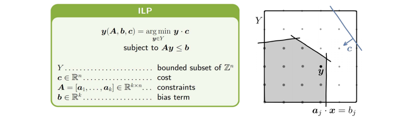

Figure 10. Definition and geometric meaning of integer programming^[16]

The equation on the left in Figure 10 is a typical form of integer programming that previously explained the knapsack problem as an example. Variable y is a variable to be determined through integer programming, belonging to the set of integers Y. The objective function y·c is defined as a linear function as the product of cost c and variable y subject to optimization, and constraint Ay ≤ b is also defined as a linear function through matrix A and vector b. The figure on the right in Figure 10 shows the geometric meaning of the objective function and constraint. The constraint expressed by linear function Ay ≤ b corresponds to the gray area in the figure. Since the boundary of the gray region consists of as many hyper-planes as the number of constraints (i.e., number of rows in matrix A), the feasible solutiony of the given integer programming can be expressed as integer values expressed in a grid within the gray area. At this point, the objective function y·c of integer programming is expressed as a blue hyperplane with a slope of c, so the y value at the point where the blue hyperplane meets the feasible solution y for the first time as it gradually approaches the gray region while maintaining slope c becomes the optimal solution we want to find. In the case of linear programming, since the variable y has real values, it can be seen that the feasible solution becomes the whole gray region, not the grids, so that one of the corner points in the gray area consisting of hyperplanes is the optimal solution. On the other hand, in the case of integer programming, it is known to be generally more difficult to obtain an optimal solution than in linear programming because the area of y of the feasible solution becomes grid points.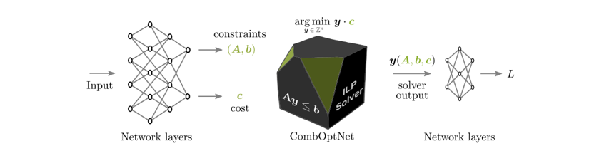

Figure 11. Schematic diagram of CombOptNet network structure^[16]

Figure 11 shows the network structure of CombOptNet proposed by the authors. c representing the objective function of integer programming and A,b representing the constraint are inferred from the input data, and optimal solution y(A,b,c) is obtained from the inferred integer programming parameter A,b,c using the mathematical optimization tool GUROBI^[5]. For the optimal solution y(A,b,c) obtained in this way, the Loss function is defined in the direction of reducing the difference from the correct answer label y so that learning can proceed. The difficulty we can think of here is that, like the Neural A* algorithm discussed earlier, the gradient for network updates is not blurred properly due to the non-differentiable nature of integer programming located in the middle of Figure 11.

Figure 12. Geometric meaning of gradient decomposition according to integer basis^[16]

To solve this problem, the authors proposed a method of decomposition of the gradient according to the integer basis as shown in Figure 12. Through this, each parameter A, b, and c of integer programming can be updated with the gradient based on the integer basis above.

Figure 13. Text-based knapsack problem^[16]

The first experiment to demonstrate the experimental performance of CombOptNet is the text-based backpack problem in Figure 13. It is the same problem as the knapsack problem described earlier, but since the input comes in the form of a sentence, an embedding network for natural language processing is additionally required. At this time, the data used for learning are the preprocessed embedding vector x for 10 items inputted in the form of sentences and the binary vector y indicating whether each item has been chosen.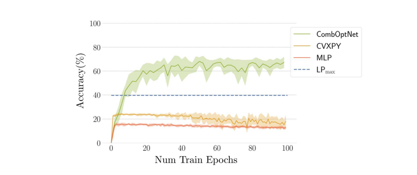

Figure 14. Comparison of the results of text-based knapsack problem experiments^[16]

Figure 14 is a comparison of the results of the text-based knapsack problem experiments above. We can see that the CombOptNet proposed in this study shows high accuracy compared to multi-layer perceptron (MLP) that performs the supervised learning base without the mathematical optimization of integer programming parameter learning, LPmax that obtains approximate solutions through relaxation to linear programming, and CVXPY, which replaces the integer programming module of CombOptNet with CVXPY^[17] based on linear programming.

Figure 15. Results of key point matching experiment^[16]

The second experiment is the key-point matching between two images. As shown in Figure 15, the relationship between the characteristic points of an animal or an object can be represented in a bipartite graph, which can be defined as a combinatorial optimization problem. CombOptNet showed that the key-point matching above is possible even for image input through integer programming parameter inference.

This study proposed a learning algorithm through explicit integer programming parameter inference and differentiable integer programming module from combinatorial optimization data for which no specific formula for integer programming is given. The biggest contribution appears to be the proposal of a differentiable network structure that can effectively solve combinatorial optimization problems in various types of data such as text and images through this. Since the optimal solution of integer programming is still calculated relying on the mathematical optimization tools, however, if the complexity of the problem itself increases, there is a possibility of the level of the optimal solution falling at the same time depending on the limitations of the mathematical optimization tool.

* Reference Paper http://proceedings.mlr.press/v139/paulus21a/paulus21a.pdf Slide https://icml.cc/media/icml-2021/Slides/9555.pdf Source code https://github.com/martius-lab/CombOptNet

So far, we have looked at two deep learning-based combinatorial optimization studies presented at ICML 2021. The combinatorial optimization problem with a discrete environment is a little unfamiliar to those who are familiar with recent deep learning-based AI research, posing a difficulty that requires thinking in a different way. Among the problems we face and solve in reality, however, there are more cases that we need to approach as a combinatorial optimization problem than we think. Optimization of production plans for various daily necessities such as parts used in the production of electronic products and groceries and optimization of proper loading and movement routes of logistics in cargo trucks or courier transportation are typical combinatorial optimization problems that remain to be solved. In addition, the combinatorial optimization problem of proper placement of electronic parts and wiring between parts in electronic circuit design is still an unsolved challenge. For these problems, I think combinatorial optimization studies based on deep learning can provide new clues to difficult problems that have not yet been solved.


ICML 2021 Review ① DiLab Kanghoon Lee  (Link)