 Hyemin Jung
2022.03.14
Hyemin Jung
2022.03.14
[NeurIPS 2021] Part 1: Generative model - Diffusion model Review
|
The Conference and Workshop on Neural Information Processing Systems(NeurIPS 2021) is a machine learning and computational neuroscience conference founded in 1987. It is also one of the most influential conferences in the field of AI and machine learning with the average acceptance rate of 20%. Here is a summary of the research papers shared at NeurIPS 2021, picked by three researchers from Applied AI Research lab, LG AI Research. - Part 1: Generative model - Diffusion model Review - Hyemin Jung from Applied AI Research lab |
Introduction
At the LG AI Research’s Applied AI Research Lab, generative models are being vigorously studied. Generally speaking, a deep learning model can be divided into two categories: discriminative and generative. Applied AI Research Lab is researching anomaly detection, representation learning, music generation, recommendation, etc. in time-series data.
The topic of this blog post touches on the subject of various generative models as well as the diffusion model, one of the most studied generative models recently. This blog will explain representative papers on diffusion model and variational diffusion model published in the NeurIPS 2021 based on said paper.
Generative model
What is a generative model?
A generative model is a model that estimates the sampled distribution of given data x. What it means for a deep learning model to estimate the distribution is that the model’s output may be the parameter for determining the distribution or the marginal likelihood of data output. A generative model can be used to determine the likelihood of test data and generate new data.
The performance of a generative model is shaped by how well it predicts the likelihood p(x) value of given data x and the quality of data x generated.
Comparison of generative models
There are 6 types of generative models. Each of their characteristics, as well as advantage and disadvantage are as follows:
Auto-regressive models(ARMs)
An ARM is the product of conditional probability of sequential variables and used to calculate the likelihood of data. Its advantage is that it can determine the likelihood of a given data and its disadvantage is its slow sampling and inability to study latent features in the data.
Variational Auto encoders(VAEs)
A VAE is a form of latent variable-based generative model that determines joint distributions of data x and latent variable z, then marginalizes data x. Its advantage is fast learning and sampling, and that the latent features of the data can be learned, while its disadvantages are intractable likelihoods and restrictive prior distributions.
Energy Based Models(EBMs)
An EBM estimates distribution using energy functions. It is simple with no constraints, but its disadvantage includes intractable likelihood and sampling.
Generative Adversarial Networks(GANs)
A GAN is a type of learning framework where the discriminator and generator contest with each other in adversarial directions and learn to generate new data. Its advantages include good sample quality, as well as fast training and sampling. Its disadvantages include undefined likelihood and unstable training.
Normalizing Flows
A normalizing flow model estimates distribution by using invertible mapping functions to transform a simple distribution, p(z), into a complex one, p(x). It can determine exact likelihoods and enables fast sampling, but its disadvantage is the limiting aspects on architectures.
Diffusion
A diffusion model estimates distribution by gradually adding noise to data x and generating noise data, then learning the process of noise data returning to data x. Although likelihoods are intractable, it has good likelihood values and can estimate complex distributions well without limitations.
Of the various generative models above, diffusion models are being heavily studied the most recently. Many diffusion models, which have better likelihood performance than autoregressive-based generative models, and generate higher quality samples than GAN-based models were published in the NeurIPS 2021.
Now, I will give a basic description of diffusion models and explain the ‘variational diffusion model,’ the diffusion model published in NeurIPS 2021.
What is a diffusion model?
Diffusion probabilistic models
The first ever paper that put forth a diffusion model was “Deep Unsupervised Learning using Nonequilibrium Thermodynamics” (2015) [1]. The idea of a diffusion model came from thermodynamics, and it can be divided into two stages. First, noise is gradually added to given data x. This process is called the “Diffusion process.” Second, the reverse process of the diffusion process defined earlier is calculated. In this process, the noise is gradually removed from the noise data transforming it into original data x. A deep learning model is used to learn this reverse diffusion process, and this process is called “Reverse diffusion process.”
1.Diffusion process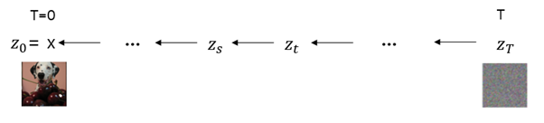
In a diffusion process, noise is added to given data x at every time step. At step 0, noise is added to move to step T, and the latent variable zt is the noise added at each step. Mathematically expressing this diffusion process gives us the Gaussian distribution as shown below:
In the equation above, the signal, is taken from the previous step, latent variable and noise, , is added to determine . Here, is the quantity of noise set by the user. As the time step gets bigger, a larger value is assigned to the noise.
Once noise is added all the way to step T, zT will eventually become an Isotropic Gaussian distribution.
A diffusion process assumes a Markov attributes. Therefore, once data x is given as a product of distribution, as shown below, the latent variable distribution can be extracted.
When data is given, the distribution of latent variable is the Gaussian distribution.
The equation above signifies specific noises added with as basis.
When are given as below using the Gaussian distributions defined above, we can deduce the Gaussian distribution of .
is the value used to determine using the reparameterization trick. This equation signifies the latent variable distribution of the previous time step, and this is important as it will serve as the solution when the model learns the reverse diffusion process.
To sum it up, a diffusion process is a course of adding noise ratio value, , at every time step and all relevant distributions can be expressed as Gaussian distributions. No learning takes place in this process.
2. Reverse Diffusion process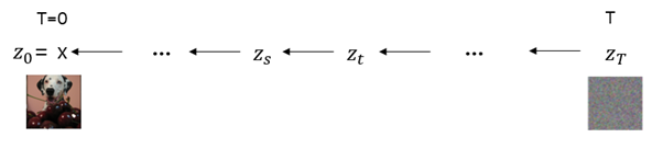
The reverse process of the former diffusion process is a generative model where the noise data return back to the original data x. Although a diffusion process is deliberately defined as a Gaussian distribution, distributions portraying the reverse diffusion process are still unknown. We can learn about unknown reverse diffusion processes through the model.
A reverse diffusion process can be expressed as the equation below:
is the reverse distribution estimated by the model. This distribution is a Gaussian distribution and the model learns the average, one of parameters of the Gaussian distribution. The equation is as shown below:
3. Loss
Let’s review the reverse diffusion process, that is, the loss equation to learn the generative model. The purpose of a generative model is distribution estimate, which can be determined by calculating the likelihood of given data x. Therefore, an objective equation must represent log likelihood of x. The loss equation can be deduced from this objective equation. The detailed process of deduction will not be mentioned here.
A loss equation is also called Variational Lower Bound (VLB) and the meaning of each term is as follows:
Because term combines two Gaussian distributions and both are Gaussian distributions, they can be calculated in closed form.
Term reconstructs the original x in latent variable z1 and this term can also be calculated directly.
Both terms above can be calculated whether the models learned it or not.
Term is called a diffusion loss and it enables the learning of the reverse diffusion process.
is the solution distribution, and it is learned to bring the model distribution ( closer to distribution. Both distributions are Gaussian distribution and KL divergence is calculated as shown below:
We have briefly gone over the concept of diffusion model and loss equations. A wide range of diffusion models have been put forth based on the information above, and many papers have been published in the NeurIPS 2021. Of the models above, I will explain the variational diffusion model.
Variational diffusion model[2]
Motivation
There have been many Diffusion models put forth with adequate performances that are based on the generated image quality, but Diffusion models based on likelihood performed poorly compared to autoregressive-based generative models. This paper proposes diffusion models that have overcome such limitations and displayed SOTA performance based on likelihood.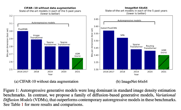
Contribution
The contributions of this paper are as follows:
- Use of Fourier feature is proposed to improve likelihood performance.
- Added noise schedule during diffusion process are determined based on how the model learns.
- Proposed a simpler form of VLB.
- Theoretically proved that the higher the number of steps is in the diffusion process, the better the performance improves.
- Deduced diffusion loss from infinite time steps (continuous time steps).
- Theoretically illustrated that the relationship between the loss equation from continuous time steps and existing diffusion models.
Forward time Diffusion process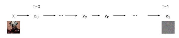
The first distribution in the diffusion process as proposed in this paper is as follows:
When data x is given, the distribution of latent variable will be a Gaussian. is the quantity of signal used from the original data x, and can be calculated after adding the noise of . αt is referred to as signal and is noise. The relationship between and is as shown below:
In this paper, a new parameter SNR(t) was proposed, which indicates signal to ratio at time t.
Greater SNR(t) value signifies more signals than noises and smaller SNR(t) value signifies more noises than signals. Therefore, SNR(t) value shrinks as t gets bigger, that is, as the diffusion process moves forward.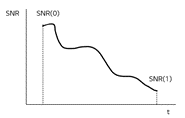
In addition, this paper proposes that noise schedule is not predetermined but learned by the models.
is a monotonic neural network model, which gives higher outputs as input, t, grows. A monotonic neural network was chosen because a diffusion process needs its data to be noisy and the noise value, , must grow. In this paper, three linear layers were used for .
Therefore, can be expressed as below:
(SNR(t) is an invertible monotonically decrease function)
The distribution comprising the diffusion process is as shown below: (0<s<t<1)
The equation signifies that, when the latent variable of the previous step is given, the distribution of the next latent variable will be a Gaussian, and that schedule information was taken at and noise was added at . The process which determines can also be deduced but it is omitted here.
Using the Gaussian distributions defined above, when given zt,x, the following Gaussian distribution can be deduced for the previous step, , as shown below:
Reverse time Generative model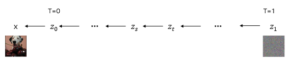
In the reverse diffusion process, original data x is generated by determining the latent variables in T=1 → T=0 direction. This process can be seen as a hierarchical generative model. There are two cases: 1) discrete time case, where there are discrete time steps with finite number of Ts between T=1 and T=0; and 2) continuous time case, where there are infinite time steps (T → ∞) between T=1 and T=0. First, discrete time case will be explained here.
Discrete time case
The span between 0 and 1 was uniformly discretized to comprise T number of time steps.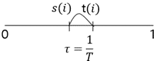
In this case, the generative model for x can be described by the following equation:
The equation above denotes that starting from noise, , and given , the outcome is , and at the model begins to return to original data x. The meaning of each term is as explicated below:
Because , is also defined as a Gaussian.
In the equation , at SNR(0), the value of is dominated by the greater value of as the noise value is small, rendering z0 and x analogous. , and element-wise scale/shift takes place when determining z0 at x, the other dimensions are not affected. Therefore, it can be defined that .
is a reverse distribution, which the model must learn. In other words,
It must learn to approach , , , distributions. distribution can be deduced in two viewpoints. First, from the viewpoint of denoising model. (Here, s(i) is s, t(i) is t.)
is a denoising model and predicts original data x once zt is entered.
Second, from the viewpoint of a noise prediction model; in the equation , when zt is calculated using the reparameterization trick, we get , . This equation can be reformulated in term of x, that is, , where can be described as shown below:
is a noise prediction model, where inputting zt predicts . In this viewpoint, is as shown below:
Denoising model viewpoint is intuitively easy to understand, but noise prediction viewpoint was applied in experiments.
Therefore, the generative model can be rearranged as shown below:
Or
Loss equation
The loss equation for learning the above generative model is as shown below:
Prior loss and reconstruction loss can be determined using the reparameterization trick. Diffusion loss is the term that can be reduced through model learning. In discrete time cases, diffusion loss equation is as shown below:
It opts to close the gap between reverse distribution of the solution and model distribution. The equation deduced from the above equation (, , ) in denoising viewpoint is as shown below:
This equation determined the difference between the actual solution x and the output after inputting latent variable zt at each step, and then weight was multiplied to the answer. A penalty was given in proportion to the difference of signal to ratio values between current and previous steps. In other words, greater penalty was given to more noisy data.
In noise prediction viewpoint, if (, , ) are expressed as SNR(t) and, is calculated using the reparameterization trick, a simple equation can be deduced, as shown below:
Continuous time case
This paper mathematically proved that diffusion loss decreased as the number of time steps increased. As such, a diffusion loss equation was deduced for the case of infinite time steps (T → ∞). In this case, t is a continuous value. A limit can be applied to the loss equation of discrete case diffusion and deduce the following equation: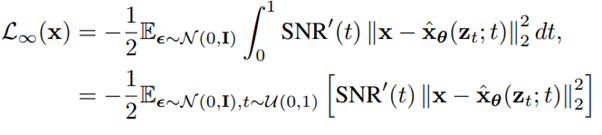
It is apparent that the weight term has been replaced by a differential value.
The equation deduced from the denoising viewpoint is as shown below: 
As mentioned earlier, a noise schedule must be learned, and therefore, the invertible monotonically decrease function, SNR(t), must also be learned. . This paper revealed through proof that in a continuous case, SNR(t) did not influence the diffusion loss equation; only SNR(0) and SNR(1) values influenced the diffusion loss. Thus, it is not necessary to learn SNR(t) parameter η to reduce the diffusion loss. Only noise prediction model parameter θ, as well as SNR(0) and SNR(1) values need to be learned.
Model parameters can be learned by calculating the equation above using the Monte Carlo (MC) estimator. The MC estimator equation is as shown below:
This paper proposes to learn parameter η of in order to reduce dispersion of the MC estimator.
Fourier Features
In summary, the generative model is as follows:
Or
There are two cases, namely discrete time and continuous time, of diffusion loss equation when learning this. Diffusion loss of discrete time case 
Diffusion loss of continuous time case (MC estimator).
In other words, the model must learn how to enter latent variable zt at each time step to predict . In this paper, in order to improve the likelihood performance, it was proposed to calculate high frequency Fourier feature of zt using the equation below
and concatenate to zt, then proceed with input. The input values for high frequency Fourier feature values have been amplified in various scales, and adding them properly captured the fine scale details.
Experiment
The VDM proposed in this paper displayed SOTA record in the likelihood benchmark compared to other generative models.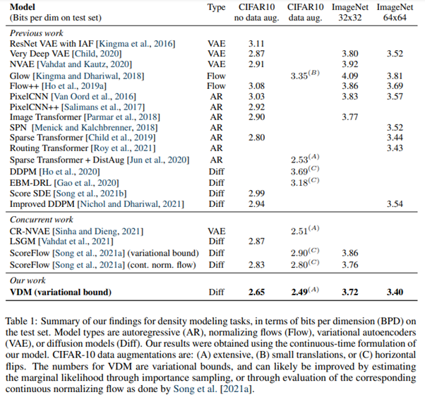
Generated image quality is as shown below: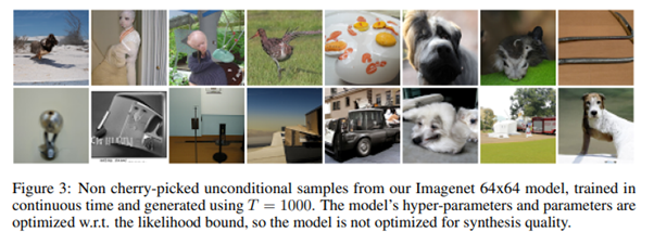
Conclusion
I have set my goal to estimate given data distributions and resolve the relevant downstream tasks. I am currently researching various generative models of images, sequential data and graph data. When writing this blog, I was able to identify the advantages of diffusion models, a type of generative model. However, the likelihood value of a diffusion model is, at the end, the lower bound value of logp(x) and a gap still exists between the two. Moving forward, I believe we need to contemplate on how to reduce this gap.
- 참고
- [1] Jascha Sohl-Dickstein, Eric A. Weiss, Niru Maheswaranathan, Surya Ganguli e “Deep Unsupervised Learning using Nonequilibrium Thermodynamics” (2015)
[2] Diederik P. Kingma, Tim Salimans, Ben Poole, Jonathan H “Variational Diffusion Models”(2021)