[NeurIPS 2021] Part 2: Variational Deep Embedding-Based Deep Clustering Review

The Conference and Workshop on Neural Information Processing Systems(NeurIPS 2021) is a machine learning and computational neuroscience conference founded in 1987. It is also one of the most influential conferences in the field of AI and machine learning with the average acceptance rate of 20%. Here is a summary of the research papers shared at NeurIPS 2021, picked by three researchers from Applied AI Research lab, LG AI Research. - Part 1: Generative model - Diffusion model Review - Hyemin Jung from Applied AI Research lab - Part 2: Variational Deep Embedding-Based Deep Clustering Review - Jinseok Yang from Applied AI Research lab - Part 3: Neural Architecture Search Review - Wonbin Ahn from Applied AI Research lab

Introduction

The Variational Autoencoder method which extracts data through unsupervised learning is used in various sectors such as Anomaly Detection, Classification, and Image Segmentation. This blog will introduce two deep clustering methods that applied variational autoencoder in clustering announced at NeurIPS 2021. For this, we will take a brief look over clustering and gain understanding on Variational Deep Embedding (VaDE)^[4], which is the baseline research for deep clustering, followed by summarizing (a) Multi-Facet Clustering Variational Autoencoder and (b) Deep Conditional Gaussian Mixture Model for Constrained Clustering announced based on VaDE at the NuerIPS.

Clustering Overview

Today’s blog will examine the deep learning-based clustering method. First, to explain why deep learning is used for clustering, we take a brief look at the basics of clustering. Clustering is a method for grouping relevant data without using labels. The most intuitive method is the similarity-based clustering that treats “data with similar appearance as relevant data.” The most famous method is spectral clustering which involves measuring pairwise distance between samples to gather similarly shaped samples. The illustration on the left side of Figure 1 calculates the distances among eight samples with similarity verification equation, $w_{i,j}=e^{{||x_i-x_j||}^2/2 {\sigma }^2}$, and demonstrates the operation method of spectral clustering that ties the samples with closest distance together. Such operation method has straightforward results and since distance between all data are verified, it has the advantage that it can properly express the groups of data that forms non-circular shape are not in their original forms- (see Figure 1 (right)). However, as the distance between all data must be measured, if there are N data, it has the weakness that it must calculate N×N distance matrices. Figure 1 expresses the similarity among the eight samples using colors. If similarity between two samples is high, the weighted value is high; if similarity is low, the weighted value is low as well.

 

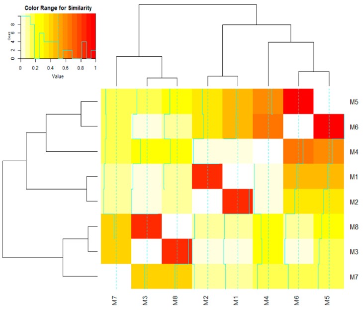
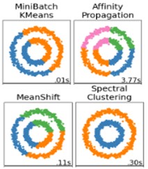
Figure 1. (Left) Spectral Clustering algorithm 0^[1] (Right) Different Clustering results

K-means is an algorithm that solves scalability issue with computation costs, and shows good clustering performance. The clustering algorithm still shows low clustering performance if there is a high quantity of data or data has missing values, but it is still currently the best known and the most used algorithm. When there is input for setting K clusters, K-means randomly selects K cluster centers (i.e. b) and calculates the distance between each data point (i.e. x_i) and K cluster centers (i.e. b) to forms K clusters which have the smallest distance between data points in each cluster and the center point as shown in the Equation 1 in below. Equation 1 is the optimization equation for carrying out K-mean using n number of data, k number of clusters, binary value w (1 if cluster exists and 0 if there are none) and set of cluster centers b (K-means solves problems through optimization, not by learning, which is why it is referred to as an algorithm). As one data must be under only one cluster, it has the restrictive condition that the sum of w for all clusters should be 1. The optimization equation includes two unknown variables, w and b, and therefore, it is impossible to optimize two values simultaneously. Thus, K-means adopts iterative approach: (i) Fix w, then optimize b and (ii) Fix b then optimize w, are performed repetitively to calculate whether the cluster center points and data are under the cluster.

Equation 1. K-means clustering algorithm to generating k clusters in n data points

As the central point of the cluster (i.e. b) is initialized randomly, it is often performed several times and then the index that evaluates whether the data are properly clustered (e.g. Silhouette Score ^[6]) is used to identify the best clustered model. K-means algorithm measures the distance between each data point and the cluster center with Euclidean metric, so the cluster forms circular shape (See Figure 2 (left)). When Norm-1 is adopted as distance metric, K-means becomes the K-median algorithm, and as square is not performed, smaller error is applied, thus making it possible for more robust clustering from the outlier.

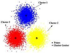
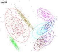
Figure 2. (Left) Example of K-means clustering results (Right) Example of GMM Mixture Model results

The Gaussian Mixture Model (GMM) performs clustering with Gaussian Mixture assumption. K-means decides which group (1 or 0) to insert each data by working the optimization equation while GMM computes the probability that each data will go into each group.

Figure 3. Graphical Model of the Gaussian Mixture Model (GMM)

The Gaussian Mixture assumption means can be interpreted asthat all data X can be is generated using from Latent z expressed with the Multivariate Gaussian. The graphical model in Figure 3 explains this. GMM is expressed as the probability that data X will be generated using the sum of multiple Gaussian PDFs as shown in Equation 2 (1). Here,π_k is the probability that the k group clusters with Gaussian Distribution will be selected. Making Training GMM to learn the distribution can be described as searching appropriate in which Gaussian Distribution with μ,Σ,π that can generate data X as shown the given data is generated, and it can be understood as the process of learning μ,Σ,π in Figure 3. The most representative GMM learning method is the EM algorithm, which but won't be discussed in explain in this blog because of space limitation.

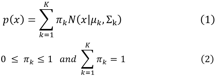
Equation 2. Mathematical formation of Gaussian Mixture Model

Deep Learning-Based Clustering (Deep Clustering)

GMM has an advantage of being able to generate clusters through learning based on data, but as expressed in Figure 3, it only has the data X generation process from latent with learned probability distribution. To explain this in further, GMM lacks the part that generates latent(the representative feature of data) from data, so it can be summarized as having limitations in forming groups that properly reflect the features of data. It is likely that better performance can be achieved by maintaining the strengths of GMM while overcoming its weaknesses. You will find the answer by checking out the graphical model of Variational Autoencoder (VAE)^[3] in Figure 4.

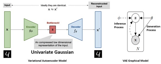
Figure 4. Structure and Graphical Model of Variational Autoencoder

VAE is an unsupervised deep learning model and it goes through a process of extracting latent (i.e. z) from the encoder(inference process), and the decoder reconstruct data from the latent z (generation process). When expressing this with a graphical model ,on the right side of Figure 4, it appears almost identical with GMM. The only difference is that an arrow from data (i.e. x) toward latent z exists. In other words, VAE can make it possible to self-extract features from data unlike GMM, and therefore, a model that merges strength of both VAE and GMM only removes the weaknesses of GMM. This method is Variational Deep Embedding ^[4] which is the basis of the two studies to be introduced today. The following is a summary of the above.

- Gaussian Mixture Model (GMM) only has a generation process that makes data, X, based on the learned probability distribution - Among deep learning models, Variational Autoencoder (VAE) can self-identify latent z with Univariate Gaussian distribution on its own - The model that combined GMM and VAE to remove the weaknesses of GMM is Variational Deep Embedding (VaDE) which is the basis for the two studies to be introduced today

Variational Deep Clustering(VaDE)

VaDE and VAE are different in the way that they extract latent. VAE presumes that latent has Univariate Gaussian as the prior, and it extracts latent directly from data. When looking at the structure of the graphical model of VAE in Figure 4, the latent z is generated directly from the data (i.e. x), and the reconstructed data(x') is regenerated from the latent z. VAE learns by minimizing the difference between the reconstructed and original data X.

Unlike VAE, VaDE generates the set of clusters with Multivariate Gaussian prior from data X, and latent z is generated from each cluster. The process for generating reconstructed signal using the decoder is the same as VAE (See Figure 5). It seems quite simple in words; then why does VaDE have research value? The reason for this is because while it does not have the method for extracting cluster c directly from data X, VaDE derives a method to replace this mathematically.

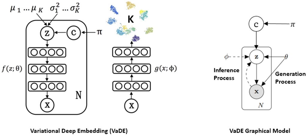
Figure 5. Structure and Graphical Model of Variational Deep Embedding (VaDE)

Research Value of Variational Deep Embedding (VaDE)

You can see the difference between the two models at a glance, when comparing the graphical models of VAE and VaDE (on the left of Figure 6) and the Evidence Lower Bound (ELBO) which described on the right side of Figure 6. For your information, ELBO must be learned toward the direction of maximizing.

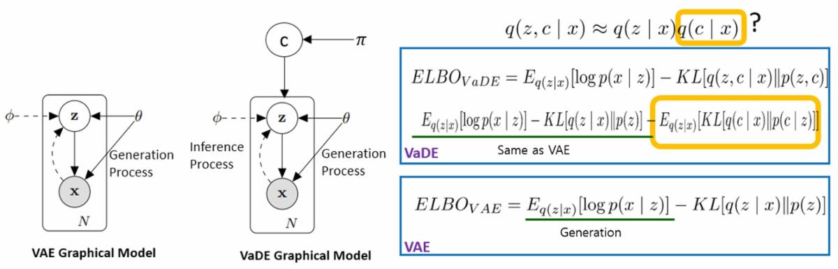
Figure 6. Difference of VAE and VaDE

The equation on the right and the illustration on the left of Figure 6 are basically the same thing. Well-trained VAE performs the generation process by utilizing the latent z which is extracted from X, and the generated X is similar to the original X. This is the first term of the ELBO equation of the VAE (ELBO_vae of Figure 6). However, the extracted latent z must have similar distribution as the prior Gaussian distribution, p(z) , that we assumed, so the expression of this is the second KL divergence term. When looking at the graphical model of Figure 6 VAE, we can see there exists only generation and inference processes, which is defined on ELBE of VAE with two terms. For VaDE, cluster C must be extracted from data X, so the final term emphasized in orange in the ELBO of VaDE is added. This term is q(c|x) and when you look at the graphical model on the left, there is no arrow that connects cluster C from data X. In other words, while it is structurally impossible to extract C from data, VaDE mathematically proves that q(c|x) is an average of the probability to generate cluster C from z as shown in Equation 3. Through such proof, we can configure VaDE by simply modifying VAE.

Equation 3. Probability to be included in cluster from data is approximately same as the average probability of extracting cluster from z

The below is a summary of the process to find VaDE using VAE.

- VaDE must extract latent z and cluster c with unsupervised learning from data - According to the VaDE Graphical Model, only x ↔ z must be connected and there is no x → c connection, and therefore, ELBO of VaDE cannot be solved. - Variational Deep Embedding (VaDE) mathematically proves that x → c probability can be solved using the z → c probability

Structure of Variational Deep Embedding (VaDE)

As VaDE is basically a variation of VAE, we will first look at the structure of VAE. VAE generates latent z with Univariate Gaussian prior assumption from data X using an encoder. Here, the Gaussian assumption of the latent z can be guaranteed through sampling, and as this is an operation that does not support back-propagation, VAE adopts Reparameterization Trick (N(0,I) part on the bottom of Figure 7). Afterwards, decoder uses the corresponding z to restore the input value.

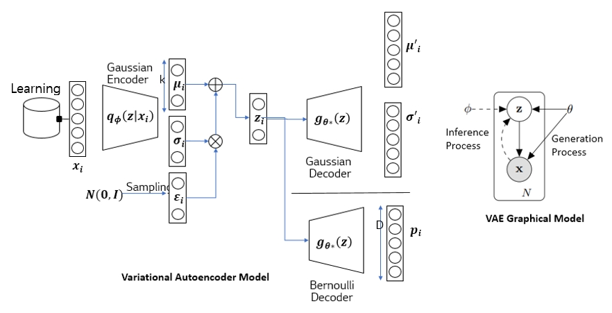
Figure 7. Detailed structure and graphical model of VAE

When looking at ELBO of VaDE (see Figure 6), C must be generated from X, but through mathematical derivation as described in Equation 3, VaDE can be configured as shown in the Figure 8 in below. It includes parts that learning the factors for clusters from latent z (see Figure 8), and as you can see that this is the only difference compared to VAE. When looking at this structure, VaDE only adds clustering parts as following mathematical derivation (see Equation 3) and it defines end-to-end deep learning-based clustering architecture.

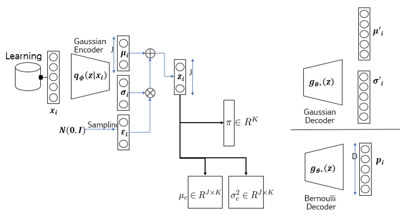
Figure 8. Detailed structure of VaDE; only part on clustering is added to VAE

Performance of Variational Deep Embedding (VaDE)

In conclusion, VAE assumes latent with Univariate Gaussian and VaDE presumes that latent is composed of the Gaussian Mixture Model. There are different features by cluster, and therefore, it is understood that clusters composed of GMM can include more various features, and this part can be confirmed through experiment results. Figure 9 compares the group performance of VAE and VaDE. In the case of MNIST, distances between clusters are farther, and when combining the cluster of different latent spaces and sending it to the decoder, as shown in the results on the right, it is evident that the image combining characteristics of two features are generated.

Figure 9. VaDE performance

Now, we will look at research on deep clustering based on VaDE presented at NeurIPS 2021. The research that will be introduced in this blog are (a) Multi-Facet Clustering Variational Autoencoder and (b) Deep Conditional Gaussian Mixture Model for Constrained Clustering.

Multi-Facet Clustering Variational Autoencoders (MFC-VAE)

You can think of this study as one that expanded VaDE. Variational Deep Embedding (VaDE) generates K-number of clusters. In other words, by grouping the data on the left of Figure 10, VaDE generates clusters for data having the same features as shown in the right image of Figure 10. In fact, like Figure 11, despite the fact the data in Figure 10 (left) can be grouped using various methods such as the “triangle, circle, square” or “red, blue, green” groups, single VaDE model can form set of clusters using just single characteristic, so called facet.

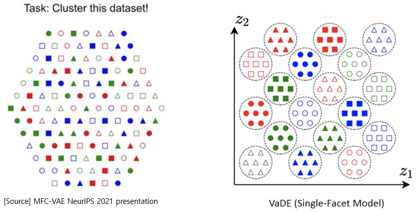
Figure 10. When multiple data are mixed together, VaDE operates as shown above

The MFC-VAE is a method that can learn all set of facets at once if data are grouped with multi-faceted methods.

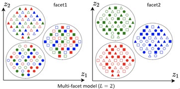
Figure 11. Example of multi-facet data.

We will explain this in a more structural way. The VaDE explained in Figure 5 extracts K-number of clusters from the data. In the case of MFC-VAE, as illustrated in Figure 12, the cluster group is defined as facet, and VaDE is expanded so that the L-number of facets composed in each K clusters can be identified through training. Graphical model in Figure 12 makes it easier to understand this concept. You can see that multi-facet clustering creates L-number of facets from the data, and each facet makes clusters separately. If you look at the graphical model on the right side of Figure 12, the part that is related to cluster creation is expressed as L. Like VaDE, graphical model of MFC-VAE has no connection from data x to cluster c. MFC-VAE overcomes this restriction by mathematically expands ELBO_VaDE to add all clustering related factors can be summed according to the number of facets.

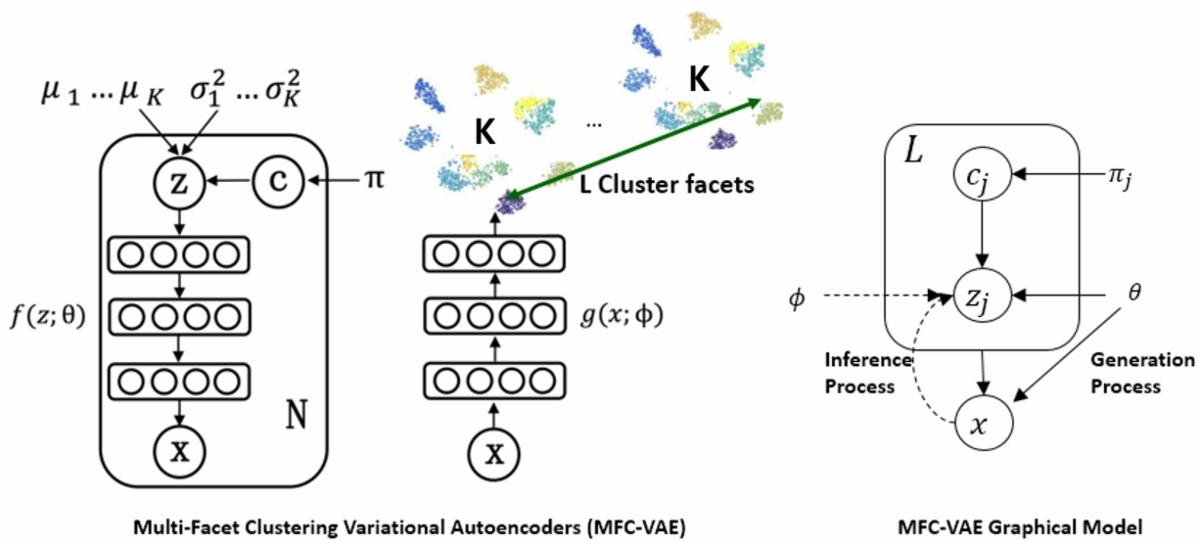
Figure 12. Concept and graphical model of MFC-VAE

We summarized In Figure 13 below, VaDE and MFC-VAE ELBO equations in were set as presumptions. VaDE ELBO in Figure 13 in below. The VaDE ELBO equation in Figure 13 is a version that expands KL Divergence Terms of ELBO_VaDE desdribed in Figure 6. is a version that develops the VaDE ELBO's KL Divergence Term. The ELBO equation of MFC-VAE is shown here, and you can see that there existsis summation only according to the number of facets in clustering related the parts having factors related to clustering. Of course, summation is also added in the fourth term, which is q(z|x), and as mentioned in Equation 3, this is because factors related to clusters are ultimately generated in latent z.

Figure 13. Difference of MFC-VAE and VAE ELBO

Due to this equation, we can now construct architecture of MFC-VAE as shown in Figure 14. When you look at Figure 14, the encoder is divided into two encoders corresponding to the base encoder and individual facet. The reason for this is that there is independent summation for each facet in the MFC-VAE ELBO equation of Figure 13, and encoder generate per facet to guarantee independence. From this context, the features of each facet are collected by the corresponding decoder, and therefore, the base decoder collected outputs from the decoders to reconstruct input.

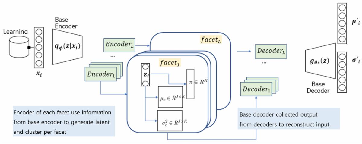
Figure 14. Detailed architecture and operation principle of MFC-VAE

Performance of Multi-Facet Clustering Variational Autoencoders

In conclusion, MFC-VAE can learn multiple types of set of clusters (i.e. facet) while conducting end-to-end training. Figure 15 summarizes the multi-facet clustering results of MFC-VAE with different datasets. The current experiment evaluates performance for two facets. For facets that emphasize shape, the same shapes are clustered, and for facets that emphasize color, those with the same colors are grouped into clusters. Although this study firmly explains contents theoretically, the reviewers presented it as the poster as it experimented only up to two facets. However, it is theoretically well summarized, and it is expected that it will also operate for more facets as well.

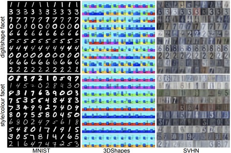
Figure 15. Clustering performance of MFC-VAE

Deep Conditional Gaussian Mixture Model for Constrained Clustering

In this paper, authors conducted research for identifying premature birth possibility using ultrasonic wave images that is provided by hospital in Germany. They discovered that when they conducted clustering, ultrasonic images with different categories were clustered together as well. In fact, medical images such as ultrasonic wave images can be interpreted by doctor as well, so it would be possible to increase accuracy of clustering if we adopt domain knowledge to cluster related images. DC-GMM is a study on how VaDE can apply domain knowledge.

Once again, we will start from the VaDE structure. The VaDE extracts clusters from input data and generates latent from each cluster. DC-GMM apply domain knowledge, called W, to the parts that extracts clusters as shown in Figure 16. The domain knowledge matrix W can be expressed as N×N matrix for N-number of data. As shown in the upper images of Figure 16, if there exists correlations between two data points, it is expressed as a positive number (must-link), and if there exists no correlation between them, it is set to be negative number (cannot-link), and 0 if there relationship is unknown. As DC-GMM well includes domain knowledge into ELBO equation of VaDE, this study was presented at NeuIPS 2021.

Figure 16. Operation principle and graphical model of DC-GMM

We compare both VaDE and DC-GMM ELBO equation on Figure 17. As you can see, the data generation process is the same, but when generating cluster, DC-GMM applies domain knowledge (underlined part of ELBO_DC-GMM) while VaDE only uses input data and latent. DC-GMM made such ELBO to be able to learn, and its details correspond to the expansion section of Figure 17. We expand ELBO equation of DC-GMM on “expansion” section, and compare to VaDE’s ELBO equation, and conclude that it is exactly same as VaDE except the part that emphasized by square at the end.

Figure 17. Difference of VaDE and DC-GMM ELBO equation

The emphasized part is basically the part that says domain knowledge must be applied when generating clusters from latent, and here, domain knowledge W is the scalar matrix in which the value is placed as a constant, and therefore, can take out. However, the constant value corresponding to the domain knowledge affects the results. In conclusion, as shown in Figure 18, the authors performed clustering by inputting domain knowledge only when computing losses at the end in the existing VaDE (see Figure 8).

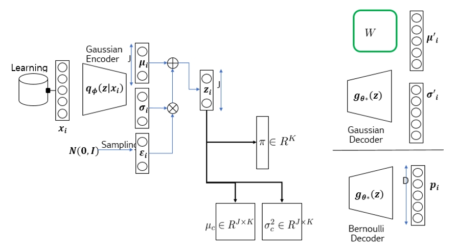
Figure 18. Detailed architecture of DC-GMM

Performance of DC-GMM

Lastly, the results show that DC-GMM shows better clustering accurately than VaDE. The test results here are facial datasets that divided Caucasians, Asians, and Indians by gender, and this is the result of entering +1, -1, 0 for correlation on 6,000 photos randomly extracted from about 20,000 photo data. The results are shown in each row, and it is evident that related faces are gathered as well.

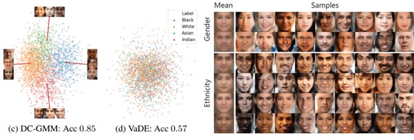
Figure 19. Performance of DC-GMM

One concern of this study is making domain knowledge matrix W. In Figure 20, authors adjust portion of pairwise correlation of data from 10% to 100%. We can observe that by entering the pairwise correlation to only 15% of data, DC-GMM only loses about 4%p accuracy compared to basic performance. However, the reviewers decided this study as the poster because it is a burden to make N×N matrix. But in the case of companies, it appears that there is little burden in making such matrices, and therefore, can be sufficiently utilized.

Figure 20. DC-GMM. Discovered that clustering accuracy increased when performing labeling between images related to 6,000 out of 20,000 images

Conclusion

This blog examined why deep learning-based clustering was proposed and how this method utilized the Variational Autoencoder. We've also looked at clustering research based on the two deep-learning methods presented at NeurIPS 2021. Because it is difficult to assess the credibility of clustering results, there is a tendency for not using this in industries that emphasize accuracy. Areas that emphasize accuracy like demand forecasting are typical areas that use supervised learning, so there is a notion that clustering cannot be used. However, problems on predicting on sales when launching new products were difficult to solve with existing supervised learning due to the lack of sales information from the past. We believe that by applying clustering to such areas to group existing sales and customer purchase tendencies, it will provide a hint for solving problems that could not be solved in the past.