Research Trends in Causal Representation Learning

Introduction

Causal inference identifies the cause of an outcome variable and infers the effect of the cause on the outcome variable. The causal inference has been gaining attention in the deep learning field because the behavior of the complex model can be understood by inferring how changing its input will affect its output. This post aims to introduce “Towards Causal Representation Learning,”^[1] which was published in the Proceedings of the IEEE in 2021.

In the machine learning field, the exponential increase in the amount of big data and advances in hardware technology have led deep learning algorithms to be applied across various fields, including natural language and image processing. In the current machine learning algorithms, a large amount of data obtained from the same independent and identical distribution (i.i.d.), are split into training and test sets, and the model is learned using the training data and evaluated using the test data. One of the main issues in the machine learning algorithms is a generalization, in which the trained models show a good performance for new data and new problems. Most machine learning algorithms ignore important data information such as the domain shift and temporal structure or regard them as unnecessary. They overcome the generalization problem by learning a model with a large amount of i.i.d data. For these reasons, the machine learning field faces several issues, which can be classified in the following three categories.

Robustness

As previously stated, most machine learning algorithms assume i.i.d data distributions; therefore, training and test sets are considered to have a similar distribution. In reality, however, they may have different distributions. For example, in computer vision, there are several reasons (e.g., camera blur, noise, and compression quality) to make a change in the data distribution. The performance of the existing machine learning algorithms may be degraded even by these simple interventions. To resolve the issue, various solutions (e.g., data augmentation, pre-training, and self-supervision) have been proposed in the machine learning field.

Learning Reusable Mechanisms

Children can understand the laws of physics in the real world by observing the consistent motion of the objects. Furthermore, they can rapidly learn something new by utilizing the previous knowledge they’ve acquired. Similarly, a machine learning model can efficiently improve its generalization performance by applying the previously-learned knowledge to new tasks. Suppose that the real world can be expressed in the modular representation and each module represents a physical causal mechanism. Then, since each module would stand for real physical mechanism, it could operate similarly across different environments and could be reused for multiple tasks without retraining. The modular system can learn new tasks quickly, whereby just a few modules are trained or added.

A Causality Perspective

Existing machine learning algorithms are based on correlation; therefore, they only understand the association between the inputs and target, and cannot infer causality between them. On the other hand, if taking a causality perspective, then the models can yield robust predictions even in various different environments from observed ones and understand the causal relations between data.

This post will explore how causality can overcome these three limitations of machine learning in the following order.

• We will first look at several methods to model real physical systems (e.g., differential equations, statistical models, and so on), and discuss each method’s assumptions and limitations. In addition, we will examine mathematical models and concepts required for causal inference, and discuss the difference between a statistical model and a causal model.
• Second, we will introduce two principles essential for estimating causal relations from data, and how they facilitate learning a causal model.
• Third, we investigate the problem of learning causal representation from data, and the current issues of machine learning algorithms will be explored from a causality perspective.
• Lastly, we will examine various problems of traditional machine learning algorithms (e.g., robustness, generalization, semi-supervised learning, self-supervised learning, data augmentation, and pre-training) from a causal language viewpoint.

 

Levels of Causal Modeling

The best way to model a natural phenomenon is to use a differential equation as follow:

Differential equations enable us to model physical mechanisms over time. Through this approach, we can predict a change in the state of the physical system, infer the effect of an intervention, and understand the statistical dependence between variables. It also provides us with physical insights and allows us to identify the causal relations between the variables.

On the other hand, statistical approaches model only the superficial part of a real system, and understand how a certain variable helps predict a target only under the same experimental conditions. Furthermore, it cannot represent a dynamic process or predict the effect of an intervention.

Causal models lie in between statistical models and differential equations. They can predict and infer the effect of interventions as in differential equation models. To predict an accurate estimation and infer such effect in the causal model, data-driven based causal discovery and causal learning approaches should be required.

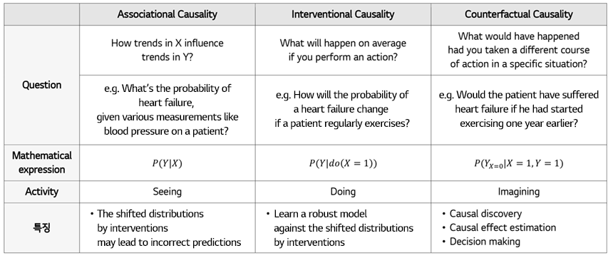
The table below shows three ladders of causation suggested by Judea Pearl^[2].

Associational Causality(Predicting in the i.i.d setting)

Statistical modeling aims to predict the distribution $P\left(Y\right|X)$, given the input X and the target Y. For example, it addresses problems like “What’s the probability of heart failure, given various measurements like blood pressure on a patient?” These problems can be solved by observing sufficiently large i.i.d. data from the distribution $P(X,Y)$. Statistical models, however, yield accurate results only in the same experiment environment, and their predictions may be inaccurate in case of the shifted distributions by the interventions.

Interventional Causality(Predicting under distribution shifts)

In a real environment, the intervention can change the data distribution $P(X,Y)$, which renders the statistical approach unreliable. In contrast, the causal learning approach can model the intervention and learn its effect, and the causal models can yield robust prediction against such distributional changes. Interventional causality deals with problems like "How will regular exercise change the patient's probability of having a heart failure?"

Counterfactual Causality(Answering Counterfactual Questions)

A counterfactual problem includes the following three fields.

• Causal discovery: The reason why the event occurred.
• Causal effect estimation: The potential outcomes if different actions had been taken
• Decision making: The actions to be taken to obtain the desired outcome. 

A counterfactual problem is a more challenging task than answering an intervention question but is an essential element of AI algorithms. Counterfactual causality addresses problems like “Would the patient have suffered heart failure if he had started exercising one year earlier?”

Causal Models and Inference

This section examines the difference between a statistical model and a causal model in more detail, and explores mathematical models necessary for causal inference and mathematical concepts like interventions and distributional change.

The Reichenbach Principle: From Statistics to Causality

Reichenbach suggests causality and statistical dependence are connected in the following way.

Common Cause Principle: if two observables X and Y are statistically dependent, then there exists a variable Z that causally influences both and explains all the dependence in the sense of making them independent when conditioned on Z.

 

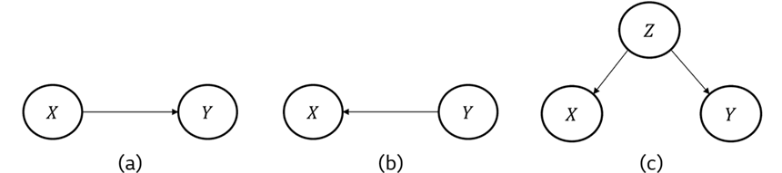
Figure 1. (a) Causal graph of $X\to Y$, (b) Causal graph of $X\leftarrow Y$, (c) Causal graph of $X\leftarrow Z\to Y$

The Common Cause Principle is illustrated by the following example, where $X$ is defined as the number of storks and $Y$ as the human birth rate. If the number of storks causes the human birth rate, the causality relation will be $X\to Y$ as in Figure 1(a); if the human birth rate causes the number of storks, it will be $X\leftarrow Y$as shown in Figure 1(b). The Common Cause Principle argues that if the two variables, $X$ and $Y$ are affected by another variable $Z$(e.g. economic growth), they will have a causal relation of $X\leftarrow Z\to Y$ as shown in Figure 1(c). On the other hand, unlike the causal graphs in Figure 1, three observational distributions of $X$ and $Y$are all identical. Therefore, one cannot distinguish the above three cases by observing the data only.  However, the causal model is particularly useful for modeling causal relations between variables to provide additional insight.

Structural Causal Models(SCMs)

This section discusses several models identifying causal relations such as causal graphical models and SCMs, and explains the key concepts of causal inference including interventions and confounders.

First of all, SCMs are represented by the observables $X_1,\cdots ,X_n$and vertices of directed acyclic graphs. $X_i$ is assumed to be in the form of a structural equation representing a causal relation between the variables $X_1,\cdots ,X_n$

$f_i$ is a deterministic function whose inputs are $X_i$’s parent nodes($\mathit{P}{\mathit{A}}_i$), and $U_i$ is unexplained random variables assumed to be jointly independent. If $U_i$ is not jointly independent, it should be another causal variable, according to the Common Cause Principle. 

Causal Graphical Model

A causal graphical model is defined as a causal (or disentangled) factorization as in (3) by exploiting jointly independent property of noise $U_i$, along with the graph structure as shown in Figure 2.

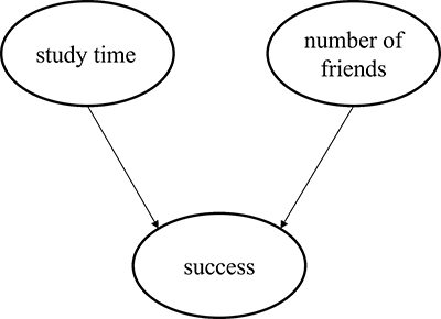
Figure 2. Example graph of a causal graphical model

In (3), $P\left(X_i\right|\mathit{P}{\mathit{A}}_i)$is considered to be a causal mechanism, and the joint distribution $P(X_1,\cdots ,X_n)$is represented as a product of the causal mechanism $P\left(X_i\right|\mathit{P}{\mathit{A}}_i)$.

Latent variables and Confounders

In the causal graphs, some unobserved variables may be contained, and the unobserved variable may affect the other two variables, which is called a confounder. In Figure 3, C represents the confounder. 

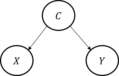
Figure 3. Confounder

Two variables affected by the confounder can be observed to be statistically related while not to be causally related. For this reason, a confounder is one of main factors that cause incorrect causal relation in the causal inference.

Intervention

An intervention refers to an operation that changes (2) by fixing $f_i$ or $X_i$ as a constant or transforming the form of $f_i$ The interventions can be divided into four categories and their descriptions are as follows.

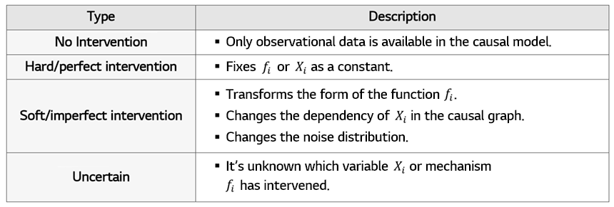
In the SCM, an intervention operation completely removes the parent node's effect as depicted in Figure 4, and it is mathematically represented by a do-operator.

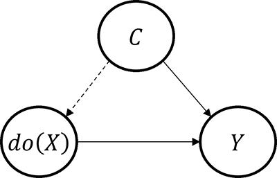
Figure 4. Intervention

Lastly, the difference between a statistical and causal model is illustrated in Figure 5.

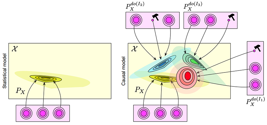
Figure 5. Difference between a statistical and causal model^[1]

While a statistical model can be represented as a single probability distribution, a causal model can be expressed as a set of various different probability distributions depending on the intervention. In summary, our goals are to identify $P\left(X_i\right|\mathit{P}{\mathit{A}}_i)$ and their relation, and to predict the effect of the intervention, counterfactual, and potential outcomes.

Independent Causal Mechanisms

This section introduces two key concepts of causality, Independent Causal Mechanisms and Sparse Mechanism Shifts. To this end, the disentangled factorization of $P(X_1,\cdots ,X_n)$ will be reviewed.

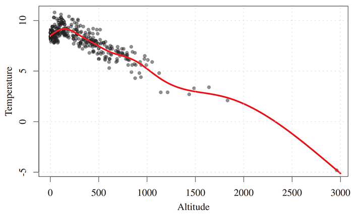
Figure 6. Data of altitude and annual average temperature^[3]

In Figure 6, we consider a data set composed of altitude A and annual average temperature $T$.The altitude $A$ and the annual average temperature $T$are related because the altitude has a causal effect on the temperature. If the altitude influences on the temperature, the causal relation can be modeled as $A\to T$and therefore becomes $P(A,T)=P(T│A)P\left(A\right)$. Since it models the natural phenomenon where the altitude affects the temperature, $P(T│A)$is (almost) always invariant in most regions. Conversely, if it is assumed that the temperature affects altitude, $P(A│T)$turns into an entangled factorization, which is no more invariant and is hard to be generalized.

Independent Causal Mechanisms

Independent Causal Mechanism (ICM) Principle: The causal generative process of a system’s variables is composed of autonomous modules that do not inform or influence each other. In the probabilistic case, this means that the conditional distribution of each variable given its causes (i.e., its mechanism) does not inform or influence the other mechanisms.

The principle of ICM involves important concepts of causality, such as the separate intervenability of causal variables; modularity of subsystems; and invariance. Applying the principle of ICM to causal factorization, the factor $P\left(X_i\right|\mathit{P}{\mathit{A}}_i)$should be independent in the following sense:

1. Changing a certain mechanism, $P\left(X_i\right|\mathit{P}{\mathit{A}}_i)$doesn't result in a change in another mechanism $P\left(X_i\right|\mathit{P}{\mathit{A}}_i)$.
2. Learning about a certain mechanism$P\left(X_i\right|\mathit{P}{\mathit{A}}_i)$$(i\ne j)$doesn’t necessarily lead to learning about another mechanism $P\left(X_i\right|\mathit{P}{\mathit{A}}_i)$.

Sparse Mechanism Shift

Sparse Mechanism Shift (SMS): Small distribution changes tend to manifest themselves in a sparse or local way in the causal/disentangled factorization, i.e., they should usually not affect all factors simultaneously.

The principle of Sparse Mechanism Shift is a result of the ICM and suggests that the small distribution changes by the intervention in the causal/disentangled factorization tends to affect few components only. This implies that if a certain intervention affects all factors, it will be difficult for the model to learn any information from the distribution changes by the intervention.

In summary, our ultimate goal is to regard the real world as a chain of an independent causal mechanism, eventually modeling it as a disentangled representation with a causal structure.

Learning Causal Variables

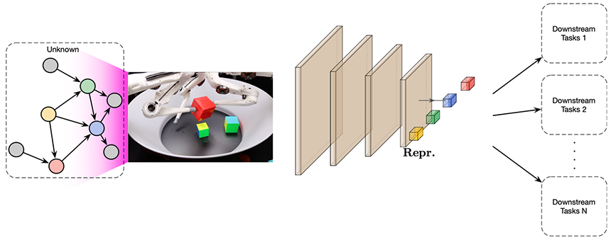
Figure 7. Problem settings of causal representation learning^[1]

Causal discovery and reasoning assume that all nodes are random variables and connected in the form of causal graphs, which implies the causal variables are known in priori. However, since most real observational data is not structured in the form of the causal variables, we need to extract causal variables from data. The relation between causal variables and observations can be modeled below.

In (4), $S_1,\cdots ,S_n$ are causal variables, and $G(\bullet )$ is a nonlinear function.As depicted in Figure 7, the causal variable $S_i$  can be extracted from the observational data $X$ through the neural network  $G(\bullet )$The main goal is to extract the causal variable $S_i$, which is usefully applied to several downstream tasks.

Learning a causal variable, on the other hand, is related to extracting robust, explainable, and fair representations from data in the machine learning field. To combine SCMs and representation learning, it requires the effort to incorporate SCMs into machine learning models. More specifically, while outputs and inputs of machine-learning algorithms are high-dimensional and unstructured, at least their insides should be designed to operate according to SCMs. The next section will discuss some problems found in traditional machine learning from the perspective of the causal representation learning.

Learning Disentangled Representations

As discussed concerning the ICM principle, the causal variables $S_1,\cdots ,S_n$ can be factorized as below, assuming that $P\left(S_i\right|\mathit{P}{\mathit{A}}_i)$is independent.

When the input data $X=(X_1,\cdots ,X_d)$is given, it’s necessary to find the causal variables  $S_1,\cdots ,S_n$and causal mechanisms $f_1,\cdots ,f_n$ modeling the causal relations between the causal variables as in (6).

This problem can be divided into the following three steps.

• Step 1: Encoder $q:$ ${\mathrm{ℝ}}^d\to {\mathrm{ℝ}}^n$, mapping $X$ to $U$
• Step 2: Mapping $f\left(U\right)$is determined by the structural assignments $f_1,\cdots ,f_n$.
• Step 3: Decoder $p:$${\mathrm{ℝ}}^n\to {\mathrm{ℝ}}^d$, mapping $f\left(U\right)$to $X$

 

Similar to auto-encoders, the above system can be learned by minimizing reconstruction errors^[4]. The majority of the research on disentanglement mostly has focused on the independent factor case, i.e., $\forall i:P{A}_i=\varnothing$Various methods^[5-7]. have been recently proposed to extract causal variables and learn the causal graphs between the variables. We refer to the corresponding papers for the interested readers.

Learning Transferable Mechanisms

The amount of data is limited in reality. If AI models work well in such an environment, they can robustly solve various real-world problems with such limited data and reuse the learned components. For this reason, the real world should be structured in the form of modular representations as previously discussed.

Implications for Machine Learning

This last section will look into the significance of traditional machine learning problems from a causality perspective.

Semi-Supervised Learning(SSL)

It is difficult to get the labeled data in reality, and labeling data should require considerable resources and costs. To address this issue, many SSL algorithms have been proposed to enhance its performance by using the unlabeled data. However, it is not yet clear exactly how the SSL algorithms work. This part will explore the SSL research from a causality perspective. We consider the causal relation of $X\to Y$as an example. The model learns mapping from $X$ to $Y$, and $P(X,Y)$can be factorized through causal factorization as below.

According to the principle of ICM, $P\left(X\right)$and $P\left(Y\right|X)$ should be independent of each other, and they have no shared information. Therefore, it is not helpful at all to use $P\left(X\right)$ to estimate $P\left(Y\right|X)$in SSL. 반면, On the other hand, learning the anti-causal relation $(Y\to X)$ can be factorized as below,

Robustness and Strong Generalization

Robustness and generalization can be considered in the form of Out-Of-Distribution (OOD) generalization, and it is possible to see the OOD problem as an optimization problem by minimizing the empirical risk in the distribution class. We consider a predictor, minimizing the empirical risk $\hat{R}$ from data distribution $P(X,Y)$.

(10) can be rewritten from the OOD perspective.

The gap between ${\hat{R}}_{P(X,Y)}\left(g\right)$ and $R_{P^{*}(X,Y)}^{OOD}\left(g\right)$ occurs from the difference between the training distribution $P(X,Y)$and the test distribution $P^{*}(X,Y)$. Looking at such OOD problems from a causality point of view, we consider the ODD  $P^{*}(X,Y)$as the shifted distribution by a certain intervention. Therefore, $P^{*}(X,Y)\in {\mathrm{\mathbb{P}}}_{\mathcal{G}}$, and ${\mathrm{\mathbb{P}}}_{\mathcal{G}}$ is a set of interventional distributions that may occur in the causal graph $\mathcal{G}$ The OOD risk $R_{P^{*}(X,Y)}^{OOD}\left(g\right)$of the worst case consequently can be defined as below.

The authors suggest that we can learn a robust predictor against OOD by minimizing the OOD risk of the worst case as follows:

Pre-training, Data Augmentation, and Self-Supervision

Since it is extremely difficult to find the exact solution of (13) for the robustness of the model, various approximated solutions will be examined from a machine-learning perspective.

• Train a model by using various and abundant data. This means that we should train a model using data obtained from diverse distributions, rather than simply a lot of samples from same distribution $P(X,Y)$.
• Train a model by using various intervention data generated through data augmentation. Then. the model can capture invariant characteristics among a range of augmented data distributions.
• Adopt self-supervision method to learn the input data distribution $P\left(X\right)$Various representations are learned through diverse data distributions  $P\left(X\right)$, which is also useful for downstream tasks.
• Train a model robust to adversarial attacks, e.g., adversarial training, etc.

The authors also recommend a future research approach to combining the above four methods (large-scale training, data augmentation, self-supervision, and robust fine-tuning).

Reinforcement Learning (RL)

RL is closely related to causality in terms of identifying the effect of interventions caused by policy. The key to learning invariance characteristic from data lies in learning from interventions. More specifically, the agent identifies the causal factor and observes its effect through interventions, and a causal model can model the environment as independent causal mechanisms. The RL problem will be examined from a causality perspective below.

Counterfactuals

A large number of samples should be required to learn RL models. Counterfactual reasoning, modeling actions in imagined space, can improve not only the data efficiency of RL algorithms but also their performance. Counterfactual reasoning is an interesting future research direction.

Offline RL

Offline RL is a paradigm that trains its policy by using only observational datasets without any interaction with the environment. To make the model work well in the offline RL, the agent can infer different actions not seen in the training data, and this is called the counterfactual inference problem. A key challenge of offline RL is a distribution mismatch between the current policy and the policy previously learned offline. The authors argue that this challenge could be overcome by learning invariant knowledge from the data with application of the ICM principle.

Multi-Task Learning and Continual Learning

Multi-task learning trains a model on various tasks in different environments, allowing it to learn common characteristics of the tasks and to efficiently learn new knowledge by applying the knowledge obtained from the previous tasks into a new task. The authors suggest that, from a causality perspective, if a causal model can learn the common data generation process of multiple tasks, it quickly adapts to shifted distribution by intervention.

Conclusion

This post examined causal representation learning, which has been gaining a lot of attention. It also proposes various approaches such as causal learning with the principle of ICM. Furthermore, it provides several solutions to enhance the performance of machine learning algorithms, whereby the problems of machine learning algorithms were examined from a causality perspective. It suggests several future research directions in causal representation learning as follows.

• Learning non-linear causal relations at scale: The high representational capacity of the latest machine learning algorithms is expected to help identify nonlinear causal relations even between many variables. Understanding what conditions enable a model to learn non-linear causal relations will also be a key research topic.
• Learning causal variables: As discussed earlier, deep-learning-based disentanglement algorithms can be used to learn the causal representations. However, even with the state-of-the-art deep learning algorithms, it is difficult to extract a dynamic disentangled representation because the extracted disentangled representation may be in random order or limited in size, which should be resolved.
• Understanding the biases of existing deep learning approaches: It is not easy to identify which component of the extracted disentangled representations is helpful for the new task. Therefore, we should understand which dataset and task facilitate downstream-task from a causality point of view.
• Learning causally correct models of the world and the agent: In RL, causal learning can be adopted for both models of the environment and the agent to obtain robust performance.

Furthermore, it is possible to apply causal representation learning to time series prediction tasks. Then, we should need to think about how to extract the disentangled causal variables in time series data. In my opinion, extracting trend or seasonality-related causal representations may be considered concerning the nature of time series data, which is also useful in downstream tasks (e.g. prediction). Furthermore, the performance of causal inference will be significantly enhanced if a human expert’s domain knowledge is employed in the causal representation learning.