[ICASSP 2023]Multi-resolution Sequence Aggregation and Model-Agnostic Framework for Time-Series Forecasting

The ICASSP (International Conference on Acoustics, Speech, and Signal Processing), considered the most prestigious conference in the field of AI for acoustics, speech, and signal processing, took place on the island of Rhodes, Greece, from June 3rd to 10th, 2023. This conference not only allows attendees to grasp the latest research trends in the field of AI-based speech and signal processing but also stages demonstrations of industry trends and technologies. This event truly serves as an active platform for speech and signal-processing experts to exchange knowledge, ideas, and professional experience.

At this conference, I had the opportunity to participate in the “Machine Learning for Signal Processing” track through the paper “Multi-resolution sequence Aggregation and Model-Agnostic framework for time-series forecasting.” It was a fruitful experience as I had the chance to exchange knowledge with numerous researchers studying in the field of AI-based signal processing. Through this blog, I'd like to briefly introduce the paper we submitted this time and share some interesting research trends that caught my attention at the conference.

Review Order I. MAMA framework: Multi-resolution sequence Aggregation and Model-Agnostic framework for time-series forecasting (Juhyun Lyu, et al., 2023)[1] II. INTERPRETABLE MULTI-SCALE NEURAL NETWORK FOR GRANGER CAUSALITY DISCOVERY (Chenchen Fan, et al., 2023)[4] III. IMPROVING WEAKLY SUPERVISED SOUND EVENT DETECTION WITH CAUSAL INTERVENTION (Yifei Xin, et al., 2023)[8]

 

I. MAMA framework: Multi-resolution sequence Aggregation and Model-Agnostic framework for time-series forecasting (Juhyun Lyu, et al., 2023)^[1]

Introduction

The “MAMA framework” is research that maximizes time-series forecasting performance by utilizing multi-resolution information inherent in time-series data. The limitations of existing multi-resolution approaches that were focused on in this paper are 1. utilizing only limited resolution information (original, down-scale), 2. during the process of merging the extracted multi-resolution information, they fails to consider the sequential order of each features, which is very important characteristic of time-series data. The contributions proposed in the paper to overcome these issues are as follows.

1. Multi-resolution input generation module: This includes not only the use of the original, down-sampled data but also the up-sampled data restored through super-resolution upsampler. This allows the use of fine detail of information that had not been used before.

2. Model-agnostic forecasting module: We can utilize the existing TSF (time-series forecasting) algorithm. We can enhance the performance of the existing TSF model by adding multi-resolution information.

3. Sequential aggregation module: During the process of aggregating and mixing the extracted multi-resolution information, it successfully preserves the sequential characteristics of the time series.

4. Multi-resolution attention fusion module: It captures and combine the major temporal dynamics of each extracted resolution signal through cross-attention.

 

Method

 

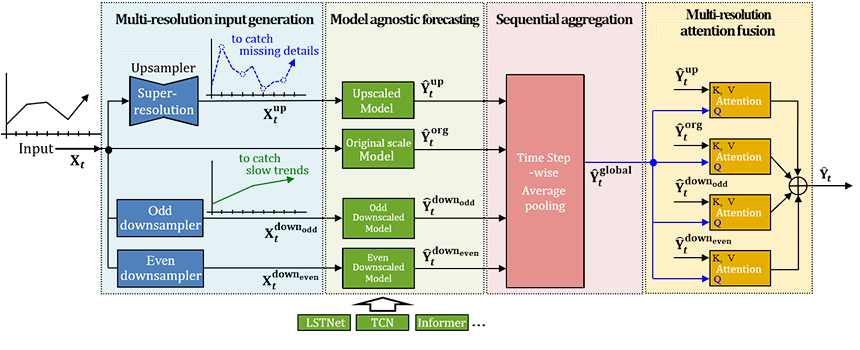
Fig. 1. Proposed MAMA framework^[1]

 

Multi-resolution input generation module

This is a module to generate multi-resolution input. Based on the input signal $X_t$, we create a high-resolution signal  $X_t^{up}$ and a low-resolution signal $X_t^{down}$ with an upsampler and downsampler respectively. Through this process, the forecasting module is able to utilize all resolution information from the original, high, and low- resolutions.

1. Upsampler : We utilized a deep learning-based super-resolution model (CNN-based U-Net structure). The reason for using the super-resolution model is to restore information of higher resolution and utilize information of fine detail for time-series forecasting. While the purpose of the existing simple interpolation technique is simply fill in the values between two values, the super-resolution model aims to restore the missing data between the two values. Thus, it was used to restore high-resolution information. The upsampling ratio of the Upsampler was fixed to 2, based on previous studies which showed significant information loss and performance degradation with upsampling ratios exceeding 2^[2].

1. - Input : ${\mathrm{X}}_{\mathrm{t}}=\{{\mathrm{x}}_{(\mathrm{t}-\mathrm{k})/{\mathrm{R}}_1},\dots ,{\mathrm{x}}_{{\mathrm{R}}_1\mathrm{t}/\mathrm{R}1}\}$

   - Output : ${\mathbf{X}}_{\mathbf{t}}^{\mathbf{u}\mathbf{p}}=\{{{\mathbf{x}}_{(t\mathit{-}k)/\mathrm{R}}^{up}}_2,\dots ,{\mathbf{x}}_{R_{2}t/{\mathrm{R}}_2}^{up}\}$

   - Upsampling ratio : $r_{up}=\frac{R_2}{{\mathit{R}}_1}=2\left(fixed\right)$

1. Downsampler : The Downsampler is used to reduce the noise in rapidly moving time series and to detect slow trends within the time series. In this paper, we adopted a downsampling method that samples data at regular time intervals. This downsampling process can induce the information loss. In order to avoid this, we adopted odd and even downsampling^[3]. To explain in more detail, we aim to minimize information loss by performing downsampling on both the odd and even sequences, as demonstrated in the data below.

1. - Odd-downsampled output : ${\mathbf{X}}_t^{{\text{down }}_{\text{odd }}}=\{{\mathbf{x}}_{t-k},\dots ,{\mathbf{x}}_{t-1}\mathbf{\}}$

   - Even-downsampled output : ${\mathbf{X}}_t^{{\text{down }}_{\text{even }}}=\{{\mathbf{x}}_{t-k+1},\dots ,{\mathbf{x}}_t\mathbf{\}}$

   - Downsampling ratio : $r_{down}=\frac{R_3}{R_1}=\frac{1}{2}(fixedforeexperimentalconvenience)$

Model agnostic forecasting module

Through this module, existing time-series forecasting models (e.g., TCN, LSTNet, Informer) can be utilized. The model in use takes information from each resolution as input and performs predictions for each scale.

1. - Input : ${\mathbf{X}}_t^{scale}$ → Output : ${\hat{\mathbf{Y}}}_t^{scale}$

Sequential aggregation module

This module aggregates outputs of different lengths from each scale to extract global information, while simultaneously maintaining sequential characteristics, thereby generating an aggregated output ${\hat{\mathbf{Y}}}_{\mathrm{t}}^{\mathrm{global}}$.

 

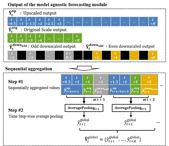
Fig. 2. Detailed operations of sequential aggregation module^[1]

1. Step #1. To maintain the sequential property, each resolution information is gathered for each time-step. For example, at an arbitrary time-step, a total of 4 values are gathered, where 2 values are from the upsample, and 1 value each from the original and downsample (Please refer to Step #1 in Fig. 2).
   
   Step #2. Apply average pooling to each group of values gathered at each time-step to extract a representative value   ${\hat{y}}_{t+\tau }^{\mathrm{global}}$ for each time-step.

1. - Time step-wise average pooling : ${\hat{y}}_{t+\tau }^{\text{global }}=\text{ AveragePool (}{\hat{y}}_{t+\tau }^{\text{up }},{\hat{y}}_{t+\tau }^{\text{org }},{\hat{y}}_{t+\tau }^{{\text{down }}_{\text{odd/even }}})$

1. Finally, we gather the representative values for each time-step to make a single sequence vector.

1. ${\hat{\mathbf{Y}}}_t^{\text{global }}=\{{\hat{y}}_{t+1}^{\text{global }},\dots ,{\hat{y}}_{t+H}^{\text{global }}\}$

1. This vector includes global temporal information, and it is used as a query for the cross-attention in the next module.

 

Multi-resolution attention fusion module

The module utilizes the cross-attention technique to leverage key information from multi-resolution signals while aligning the prediction length. In this case, ${\hat{\mathrm{Y}}}_t^{\mathrm{global}}$, which has the same length as the final output, is used as the query, and each resolution prediction output is used as the key and value. Finally, we derive the final output by summing the outputs from each scale.

1. - Attention output : ${\mathbf{A}}_t^{\text{scale }}=cross\text{-attention (}{\hat{\mathbf{Y}}}_t^{\text{global }},{\hat{\mathbf{Y}}}_t^{\text{scale }},{\hat{\mathbf{Y}}}_t^{\text{scale }})$

   - Final prediction output : ${\hat{\mathbf{Y}}}_t={\mathbf{A}}_t^{\mathrm{up}}+{\mathbf{A}}_t^{\mathrm{org}}+{\mathbf{A}}_{\mathbf{t}}^{{\text{down }}_{\text{odd }}}+{\mathbf{A}}_t^{{\text{down }}_{\text{even }}}$

EXPERIMENTAL RESULTS

For performance validation, we used real-world datasets commonly used in the field of time-series forecasting, such as ECL, Solar, and PEMS04. We used MSE, MAE, and, $R^{2}score$ as metrics.

 

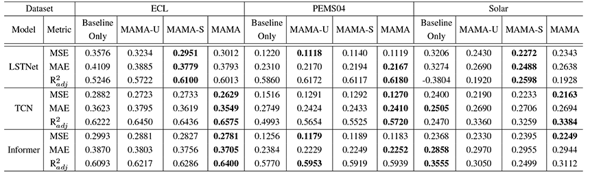
Fig 3. Multivariate time-series prediction result of MAMA
using MSE, MAE, and adjusted R2 score as metrics^[1]

 

Through the experiment, we evaluated the performance of the following 1. the performance of the MAMA framework, 2. the performance depending on the presence or absence of upsampling information, and 3. the performance depending on the presence or absence of sequential aggregation.

 

Baseline only vs. MAMA framework

Through Fig 3, it can be observed that, in the sense of MSE, the prediction performance has improved in almost all baselines and datasets where MAMA has been applied.

 

Upsampling

Based on MSE, it can be confirmed that including upsampling information yielded better performance in almost all cases than without upsampling (MAMA-U). This shows that the detailed information obtained through upsampling enhances the prediction performance.

 

Sequential aggregation (SA)

We can see that in almost all cases, the performance is superior when SA is included compared to when it is not, in the sense of MSE. This confirms that SA effectively preserves the sequential characteristics and improves the prediction performance.

 

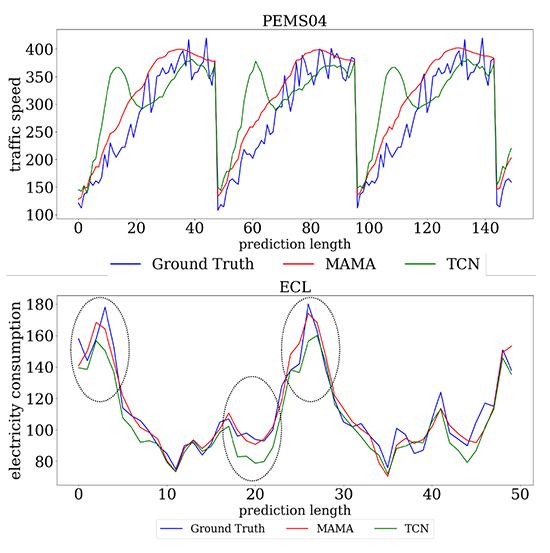
Fig. 4. Prediction result of MAMA and baseline models^[1]

 

In addition, in case of PEMS04 dataset at Fig. 4, MAMA is more accurate than baseline TCN for identifying seasonality. Furthermore, in the case of ECL, it can be observed that the MAMA identifies signal peaks more accurately than TCN. This is attributed to MAMA's utilization of fine-grained information from upsampling, enabling it to better track the peaks.

 

Conclusion

This paper proposed a MAMA framework, which can improve the performance of time-series forecasting by fully utilizing multi-resolution information based on existing time-series forecasting models. The proposed model allows for the restoration and utilization of the fine-detail information from upsampling, and it also offers a way to integrate information without compromising the sequential property of time-series during the process of merging multi-resolution information.

During the presentation of this paper at the conference, we received various feedback such as questions about the signal processing perspective and questions about the machine learning techniques used. Among these, one of the most frequently asked questions was about the practical application of the proposed algorithm. In reality, we applied the MAMA framework in stock price forecasting and demand forecasting projects. Especially, we were able to attract people’s attention when we explained that it was used in the M6 competition which ran from last March to this January for forecasting the prices of stocks.

Furthermore, there's a consistent feedback we have been receiving from our clients while conducting various demand forecasting tasks. From the client's perspective, they were curious about the cause of the prediction result, in other words, why such a result was derived. This has been one of the major feedback from clients. We believe this kind of feedback is crucial as it is directly linked to the reliability and usability of the project results. Researchers at LG AI Research also recognize the importance of this feedback and are currently conducting causal inference research to identify and explain the causes behind certain phenomena. I am also conducting causal inference research in order to address these issues.

Causal inference is a field of research aimed at inferring and understanding the causal relationships behind the certain phenomena. One can say that it mainly focuses on understanding the way in which a result occurs due to a certain cause based on data or observations and identifying causal connections (causal discovery). Based on this, the research into inferring potential outcomes depending on changes in causal variables (treatment effect estimation), and designing which causal factor to change in order to achieve the desired outcome (causal decision making) are also representative areas of research in causal inference.

Not only the field of AI-based signal processing that I attended in this conference, but I also paid close attention to research related to causal inference. Causal inference is a field that is attracting a lot of attention recently, a variety of studies related to this field were also introduced in the ICASSP. Among these, I would like to introduce two of these studies: 1. Causal discovery research to extract causal relations from a multivariate time series, and 2. A research that causal inference is applied to the field of speech signal processing from an application perspective.

 

II. INTERPRETABLE MULTI-SCALE NEURAL NETWORK FOR GRANGER CAUSALITY DISCOVERY (Chenchen Fan, et al., 2023)^[4]

Introduction

This research aims to discover causality in multivariate time series by using Granger causality, which has been widely used for a long time. For this purpose, they propose a new multi-scale neural network model called MSNGC (Multi-Scale Neural Network for GC Discovery). Summarizing the methods proposed through MSNGC in the paper:

1. They introduced a structure that avoids data segmentation between input time-series and time lags, enabling the capture of complete causal relationships among all time-series and providing an accurate binary causal graph.

   For enhancing interpretability, the paper also proposes:

2. A consistency-based thresholding algorithm for binary causal graph inference,

3. A positive/negative effect sign inference method to detect the effect sign between nodes,

4. A self-adaptive lag discovery algorithm to identify delayed time points.

 

Proposed Methods

Architecture

In this paper, the authors propose a novel architecture that maximizes the utilization of multiple time lags in multivariate time series inference. This design aims to avoid explicit data segmentation between series and time lags, as mentioned earlier.

 

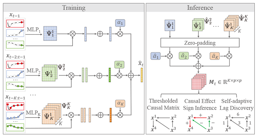
FIg. 5. The framework of MSNGC^[4]

 

The proposed model is composed of $K$ branches. Each branch takes in $p$ time series data as inputs, with lag values ranging from $t-1$ to $t-k$. The number of branches $K$ acts as a receptive field controller, adjusting the data range that each branch can examine. By considering multiple branches simultaneously, the model avoids the need for explicit data segmentation.

The model's architecture, illustrated in Fig. 1, can be formulated as follows:

 

Each $K$th branch uses an MLP (Multi-Layer Perceptron), and its output is represented as ${\mathbf{\Psi }}_k^t=\left({\Psi }_k^1\right|\cdots \left|{\Psi }_k^k\right)\in {\mathrm{ℝ}}^{k\times p\times p}$. In ${\mathrm{\Psi }}_k^l\left({\mathit{x}}_{t-k:t-1}\mathbf{\right)}\in {\mathrm{ℝ}}^{p\times p}$, $l$ represent the lth time lag, and k denotes not only means the kth branch but also indicates that it includes up to the kth time lag. The indexed element (l, i, j) of ${\mathit{\Psi }}_k^t$represents the causal effect strength from the  i-th variable to  the j-th variable at lag i.

The output of Eq. (1) $\sum _{1\le \mathrm{l}\le \mathrm{k}}{\mathrm{\Psi }}_k^l\left(x_{t-k:t-1}\right)x_{t-l}$, aggregates information across different time lags within the K-th branch. The output values from K branches are processed using a weighted sum where weights ${\alpha }_k$ are generated using a different neural network. In summary, the model examines each time series and its associated time lags together to extract information effectively. The loss function for training the model is defined as follows: 

where $R({\alpha }_k,{\mathbf{\Psi }}_k^t\mathbf{)}=\mu \parallel {\alpha }_k{\mathbf{\Psi }}_k^t{\parallel }_1+(1-\mu )\parallel {\alpha }_k{\mathbf{\Psi }}_k^t{\parallel }_2^2$ and, by setting μ = 0.5 to achieve both sparsity and smoothness. The three terms of the above Loss were designed for forecasting performance, regularization, and temporal smoothness, respectively.

 

Granger causality inference

To obtain the Binary Causal Graph B after model training, the following steps are taken:

1. Initialization Phase: Generation of the weighted matrix eighted matrix $A_k$

   In the initialization phase, the predicted output t ${\hat{\mathrm{\Psi }}}_k^t$ and the learned attention weight ${\overbrace{\alpha }}_k$ are processed to create the unsigned weighted adjacency matrix $A_k$. First, the dilated version of  ${\hat{\mathrm{\Psi }}}_k^t$ is obtained by zero-padding, represented as ${\stackrel{\circ }{\mathit{\Psi }}}_k^t\in {\mathrm{ℝ}}^{K\times p\times p}$. Then, the information from K branches is combined with the weight ${\overbrace{\alpha }}_k$to form ${\mathit{M}}_t=\sum _{k=1}^K{\hat{\alpha }}_k{\stackrel{\circ }{\mathbf{\Psi }}}_k^t$. Then, if only the causal signal strength is of interest, the unsigned weight adjacency matrix  ${\left({\tilde{\mathit{A}}}_k\right)}_{i,j}={median}_{K+1\le t\le T}\left|{\left({\mathit{M}}_t\mathbf{\right)}}_{k,i,j}\right|$ can be obtained. On the other hand, a signed matrix ${\overline{A}}_k$can be obtained by removing the absolute value. Here, ${\left({\tilde{\mathit{A}}}_k\right)}_{i,j}$ represents the causal effect strength from the j-th variable to the i-th variable at lag k. These matrices capture the causal relationships with respect to the time intervals for each lag.
   
   Next, the thresholding algorithm for inferring the Binary Causal Graph B is as follows.
   
   

2. Generation of Weighted Matrix C

   The weighted matrix C is constructed by taking the maximum values among K weighted matrices ${\tilde{A}}_k$, i.e.,

   
   
   

   For instance, $C_{i,J}$ represents the maximum GC strength from $x_i$ to $x_j$.
   
   

3. Generation of Binary Matrices ${\mathit{U}}_{\mathbf{q}}$and $\widetilde{{\mathit{U}}_{\mathbf{q}}}$

   Each binary matrix $U_q$ and $\widetilde{U_q}$ are binarized matrices based on causal metrices C and $\tilde{C}$ (which is generated from reverse chronological order of C)^[5], and its threshold set $C_{{\xi }_q}$ and ${\tilde{C}}_{{\xi }_q}$, for a specified quantile ${\xi }_q$. They can be defined as ${\mathit{U}}_{i,j}^q=\mathrm{𝕀}({\mathit{C}}_{i,j}-C_{{\xi }_q})$ and ${\tilde{\mathit{U}}}_{i,j}^q=\mathrm{𝕀}({\tilde{\mathit{C}}}_{i,j}-{\tilde{C}}_{{\xi }_q})$, where threshold values $C_{{\xi }_q}$ and ${\tilde{C}}_{{\xi }_q}$ are the thresholds for quantile  ${\xi }_q$. These quantiles are chosen based on consistency in causal inference results.
   
   

4. Generation of Binary Causal Graph B

   The Binary Causal Graph B is generated based on the optimal quantile ${\xi }^{*}$. Here, ${\xi }^{*}$ is selected as the one that shows the highest consistency from $U_q$ and $\widetilde{U_q}$. That is, it is chosen based on whether the results of the causality inference are consistent. The process of finding the optimal quantile ${\xi }^{*}$involves calculating the balanced accuracy (BA)^[6] and the Levenshtein distance (${ϵ}_q$)^[7] which is for complementing the limit of BA. Then through these the consistency score $({\tau }_q=BA-{ϵ}_q)$is calculated. The optimal quantile ${\xi }^{*}$ is selected with the quantile level with the highest consistency score. By iterating through the process of selecting the optimal quantile level, the final Binary Causal Graph B is obtained.

Causal Effect Sign Inference

Next, this paper provides the sign (positive/negative) of the causal effects for the interpretability. Based on the previously obtained weighted adjacency matrix ${\overline{\mathit{A}}}_k$, the causal effects are computed, and a positive sign indicates a positive causal relationship, while a negative sign indicates a negative causal relationship.

 

Self-adaptive Lag Discovery

Lastly, the Self-Adaptive Lag Discovery algorithm is utilized to estimate the causal lag of each cause-effect pair. This process extracts information from the unsigned weighted adjacency matrix ${\tilde{A}}_k$.

To briefly explain the Self-Adaptive Lag Discovery algorithm, it divides the input vector into two groups based on a specific index. Then, the absolute element values within each group are compared. By repeating this process and finding the index c* that maximizes the difference between the two groups, the optimal time lag is determined. In other words, this algorithm identifies a significant point where the difference between the two groups is most pronounced, which allows for meaningful interpretation of causal relationships.

In summary, the Self-adaptive Lag Discovery algorithm helps discover the optimal time lags by finding critical points in the differences between two groups, enabling meaningful interpretation of causal relationships.

 

Experiments

In this paper, the proposed methods were validated through experiments, aiming to demonstrate three key aspects. Firstly, the accuracy of the binary causal matrix B was used to evaluate the ability of causal graph inference. Secondly, the ability to infer causal-effect signs was evaluated. Lastly, the lag discovery ability was compared with existing models.

The metrics employed for evaluation included accuracy (ACC), balanced accuracy (BA), which considers class imbalance, and widely-used AUROC and AUPRC for binary classification performance assessment.

 

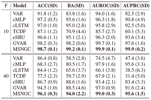
Fig. 6. Performance comparison on the Lozenz 96 data^[4]

 

Inferring Causal Structure

To evaluate the ability of causal structure inference, the data from the dynamic system Lorenz 96 model was used. The complexity of the model was controlled by adjusting the chaos variable F. The proposed model, MSNGC, was compared with other models in terms of causal structure inference. The results in Fig. 6 demonstrate that the proposed model outperforms other models in all metrics regardless of the level of chaos.

 

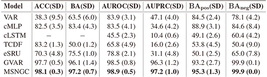
Fig. 7. Result on muti-species Lotka-Volterra data^[4]

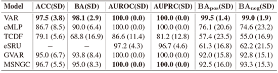
Fig. 8. Performance comparison on the VAR data^[4]

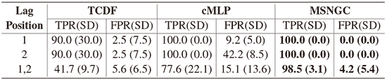
Fig. 9. Performance comparison for lag discovery^[4]

 

Inferring Causal Effect Sign

To assess the ability of causal-effect sign inference, Lotka-Volterra and VAR data were used. As shown in Fig. 7, the MSNGC model exhibits superior performance in all measurement metrics for the Lotka-Volterra data. In the case of VAR data, as expected, the VAR model performed the best. However, excluding the VAR model, the MSNGC model shows better performance compared to other models, as depicted in Fig. 8.

 

Lag Discovery Analysis

For lag discovery, the lag position is altered to compare the TPR and FPR accuracy with other models. The results in Fig. 9 indicate that the MSNGC model demonstrates the most exceptional performance compared to other models in terms of lag discovery.

 

Conclusion

In conclusion, this paper proposes a novel approach for Granger causality discovery using a multi-scale neural network. The model avoids explicit data segmentation between time-series and time lags, and capturing complete causal relationships among all time-series and providing accurate binary causal graphs. Additionally, interpretability is ensured by inferring causal effect signs and identifying the most influential time lag.

The proposed methods are significant in addressing the challenging task of discovering causal relationships in multivariate time-series data, which has been a persistent issue in the field of causal discovery. And the consideration of causal effect sign inference and the identification of the most impactful time lag added for the usability of the model.

However, it should be noted that the resulting causal graph is a binary matrix, which limits the amount of information conveyed. Furthermore, the limitation imposed by the number of time-series data points (K = number of nodes in the graph) indicates an area that requires further investigation in future studies.

 

IMPROVING WEAKLY SUPERVISED SOUND EVENT DETECTION WITH CAUSAL INTERVENTION (Yifei Xin, et al., 2023)^[8]

This study addresses challenging issues in weakly supervised sound event detection (WSSED) using the concept of causality.

Introduction

First, let's define the weakly supervised setting for sound event detection (SED). In SED, a weak label refers to an audio clip level label, not a frame level label (from a time-scale perspective, a clip is a larger unit than a frame). The weak label indicates whether the specific audio clip contains a certain audio event. Therefore, weak labels provide information about the presence of audio events in broader categories, rather than precise temporal localization.

The paper introduces the CI-WSSED, a novel network architecture with causal intervention, to resolve the “entangled context” problem in WSSED caused by weakly supervised training. The “entangled context” refers to the issue where the model learns incorrect correlations due to frequent co-occurring sound events and background sounds. For instance, sound events like “train” and “train horn” often occur simultaneously, and the model may associate them as the same class, leading to interference in sound event recognition and detection. Similarly, when background sounds are present during sound event occurrences, entangled situations arise,

To address this problem, the paper focuses on:

1. Identifying the “entangled context” problem in WSSED from the perspective of entangled co-occurring sound events and background sounds.

2. Introducing the concept of causal intervention to WSSED and proposing the CI-WSSED network structure, which integrates causal intervention into the WSSED pipeline in an end-to-end manner.

3. Demonstrating the performance improvement of CI-WSSED through various experiments.

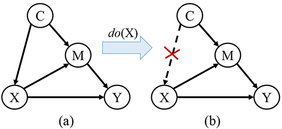
Fig. 10. (a) The structural causal model (SCM) for WSSED.
(b) The intervened SCM base on backdoor adjustment for WSSED^[8]

 

CAUSAL INTERVENTION

In this paper, the authors adopt causal Structural Causal Models (SCMs) and causal intervention to address the “entangled context” problem in Weakly Supervised Sound Event Detection (WSSED). SCM is a model that represents causal relationships in a graph format, where nodes represent probabilistic variables, and directed edges depict the causal relationships between variables (Fig. 10, SCM example).

Next, the concept of causal intervention (do-calculus) was introduced. Causal intervention aims to clarify the causal relationships between causes and effects by controlling ambiguous factors through intervention (backdoor adjustment) and focusing only on the fundamental causal relationships. Mathematically, it is represented by eq. (1), where the variable X is fixed to a constant x to make X independent from its parent nodes (causes) (Fig. 10 (b)).

Such interventions can be used to block the influence of confounders that cause confusion in finding causality and concentrate on identifying true causality. In this paper, causal intervention is applied to resolve the “entangled context” problem in WSSED.

 

Proposed Method

Structural Causal Model for WSSED

Through SCM, the paper explains how the “entangled context” in WSSED adversely affects the classification and localization performance of sound events. To understand this, let's first summarize the meaning of each node and their relationships in the graph shown in Fig. 10:

1. X: It refers to the root cause we are looking for, and in this context, it refers to the frame-level features of the sound event we are trying to identify.

2. C (confounder) → X: Here, C refers to a confounder, and in WSSED, it refers to “contextual bias.” The confounder refers to a variable that is related to both the independent and dependent variables but does not have a direct causal relationship. It acts as a disturbing variable that confuses the direct cause of a phenomenon. In the context of WSSED, C represents the “entangled context” that occurs when multiple sound events co-occur. For example, when both “train” and “train horn” sound events occur simultaneously, the model may form incorrect associations between these two events, leading to difficulties in sound event recognition and detection.

3. X → M (mediator) → Y: From a causal perspective, M stands for the mediator, which represents an intermediate variable between the cause and the outcome variable. In this paper, M represents the X-specific context formed by the combination of frame-level features X and entangled context C. In other words, M acts as an intermediary in the causal relationship between X and Y (the predicted clip level label), demonstrating that the recognition of any sound event includes the influence of concurrently occurring events.

4. Y: This refers to the outcome, and in this case, it refers to the predicted clip-level sound event label.

5. X → Y ← M: This connection indicates that the sound event X  and the mediator M  jointly influence the final prediction.

Causal Intervention via Backdoor Adjustment

In this paper, the authors propose a method for backdoor adjustment through causal intervention to control backdoor paths. Backdoor paths refer to paths in causal relationships that are not directly influenced but effects through intermediate factors. Referring to Fig. 10 (b), backdoor adjustment is used to remove the confounder and block the backdoor path to find the relationship between X and Y.

To perform backdoor adjustment, C is first separated into various class contexts $C=\{c_1,c_2,\dots ,c_k\}$ and the do-operation is used to block the link between C and X. Separating C into class-level contexts is done to handle simultaneously occurring classes independently to address the entangled context problem. Backdoor adjustment can be represented by the following equation.

 

 

Here, $f(x,c_i)$represents M, which is formed by the combination of X and C. The above equation requires k times of forward path propagation, resulting in a significant cost. To address this issue, the authors simplify the equation using the Normalized Weighted Geometric Mean (NWGM)^[9]. NWGM is a weighted average method used to approximate the expectation value in backdoor adjustment. Here, it is used to approximate $P\left(Y\right|do\left(X\right))$by moving the external sum $\sum _i^{n}P\left(c_i\right)$ of eq. (2) to the feature level.

 

 

By using NWGM, the equation is simplified, requiring only one forward pass. Additionally, the paper assumes that each class has an equal number of samples, leading to further simplification of the approximated equation:

 

 

In the equation above, $x\oplus \frac{1}{k}\sum _i^{k}f(x,c_i)$represents the projection of X, which means applying the context information of each sound event class to X while maintaining the original features. In other words, the simplified backdoor adjustment equation considers all k class contexts while augmenting the features of X through its projection, making the event boundaries clearer.

 

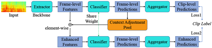
Fig. 11. Overview of our proposed CI-WSSED approach^[8]

 

Network Structure

In this paper, the causal intervention for WSSED is implemented through a network structure called CI-WSSED. Fig. 11 illustrates the process. Firstly, the feature extractor (based on CNN, RNN, or Transformer) initially takes the mel-spectrogram as an input and generate high-level feature $X\in {\mathrm{ℝ}}^{c\times n}$. Here, c is the number of channels and n is the number of audio frames. Next, X goes through the classifier and frame-level prediction before being aggregated to generate clip-level predictions. Here, the part that implements the causal intervention process of eq. (4) is the context adjustment pool Q. According to eq. (4), Q continuously stores the context information of each occurring sound event and projects it back to the X generated by the backbone to create enhanced features $X^e\in {\mathrm{ℝ}}^{c\times n}$.

 

 

Here, BN refers to batch normalization, j represents the class index of the sound event in each audio clip level label, and λ indicates the update rate. The enhancement of features at the frame level can be defined as follows.

 

Here,  ⊙ represents the matrix’s dot product, and Conv denotes a 1×1 convolution. Not only can this mitigate the impact of the entangled context, but also by focusing on the active region of the frame level feature, it can reduce the classification error and improve the localization performance. Lastly, the loss function is defined as follows.

Here, $s^{*}$represents the actual labels of the audio clip. Here, a shared weight is used for the two classifiers, where the first classifier generates an initial prediction score $S=\{s_1,s_2,\dots ,s_k\}$, and the second classifier generates a more accurate prediction score $S^e=\{s_1^e,s_2^e,\dots ,s_k^e\}$ using enhanced frame-level features. Then, the cross-entropy loss for the two classifier branches is optimized and trained together end-to-end.

 

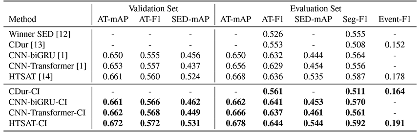
Fig. 12. Performance comparison of CI-WSSED and baseline models
on the DCASE2017 task 4 validation and evaluation set^[8]

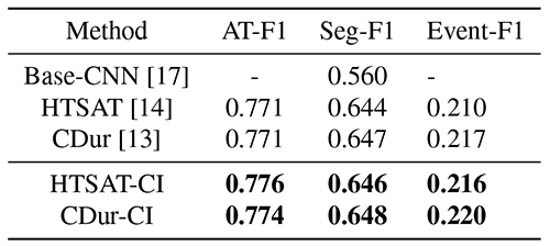
Fig. 13. Performance comparison of CI-WSSED and baseline model
On the weakly labelled UrbanSED test set^[8]

 

EXPERIMENTS AND RESULTS

In this paper, two SED (Sound Event Detection) datasets, task4^[10] and UrbanSED^[11] datasets, are used for the experiments. DCASE2017 task4 is a Large-scale WSSED dataset for smart cars, while UrbanSED is a dataset consisting of 10 event labels in urban environments.

To evaluate the effectiveness and generalization ability of CI-WSSED, the authors applied the CI-WSSED method to various baseline systems and compared their performances. The evaluation metrics used were audio tagging mAP (mean average precision), audio tagging F1 score, sound event detection mAP, segment-F1 score, and event-F1 score.

 

Results

FIg. 12 shows the experimental results from DCASE2017 Task 4, and FIg. 13 shows the experimental results from UrbanSED. “baseline-CI” represents the baseline system with the causal intervention method applied.

The experimental results consistently showed a performance improvement of CI-WSSED across all baselines. Particularly, the improvements were more significant in mAP, AT-F1, and Event-F1 metrics for DCASE2017 Task4. However, the performance improvement in UrbanSED was not as distinct. This is attributed to the presence of many sound event classes that coexist, such as “train” and “train horn,” in the DCASE2017 Task4 dataset, leading to a greater influence of “entangled context” and hence greater advantages of CI-WSSED.

 

CONCLUSIONS

This paper proposes the CI-WSSED method as a solution to the “entangled context” problem in WSSED tasks. To address this issue, the authors define the “entangled context” situation in WSSED tasks using SCM (Structural Causal Model) and implement it as a network through causal intervention techniques.

While this paper does not cover many cases or achieve significant performance improvements in WSSED, what makes it particularly interesting is the introduction of causal concepts to overcome limitations in scenarios with limited information. It demonstrates the potential to approach problems where data and information are limited.

Among the previously introduced studies, 1. The research on causal discovery for multi-variate time-series data is currently one of the main research areas within LG AI Research. In fact, interpreting causal relationships in multi-variate time-series is a challenging task as it requires considering not only the causal relationships between variables but also their changes over time. It is an interesting research to refer to as it deals with a common research topic. Among the points focused on interpretability, the part where the model identifies the time lag with a representative causal relationship is considered to be a relevant research topic for future reference in terms of enhancing the interpretability of the model.

The second study on WSSED, which introduces causal concepts to solve the problem, is valuable from an application perspective. Indeed, apart from discovering causal relationship (causal discovery), interpreting it and figuring out how to use it is another challenge. I think this research can serve as a reference for future studies on causal relationship interpretation and treatment effect estimation, where treatments are applied to causal variables to achieve desired results.

▶ Multi-Resolution Sequence Aggregation and Model-Agnostic Framework for Time-Series Forecasting (Link)