The future of forecasting and the M6 competition conference

Photo 1. The future of forecasting and the M6 competition conference
ⓒhttps://mofc.unic.ac.cy/

The Future of Forecasting and the M6 Competition Conference was held in New York, USA on November 6-7, 2023. The Demand Forecasting Squad of LG AI Research's Data Intelligence (DI)  Lab was invited to participate in the M6 Competition as a winner of three awards. Held by the M Open Forecasting Center (MOFC), which organized the M6 Competition, the conference is significant because it deals only with issues related to forecasting. The two-day program consisted largely of presentations of the outcomes of the Competition and winning methodologies as well as the sharing of insights with forecasting experts from academia and industry. Despite differences in the kinds of data that they dealt with, participants shared very in-depth knowledge as they were engaged in the same field of work and research – forecasting. In addition to this, all the participants were tackling similar challenges – from AI-enabled demand forecasting to finance – to those that LG AI Research is working on, so we could share diverse approaches and gain useful insights.

The conference consisted of several sessions and panel discussions, which could be classified into two main topics: 1) M6 competition review and 2) time series forecasting. The Competition sessions examined the summary of results and hypotheses based on Competition outcomes and the reports submitted by the participants and identified differences between theories in existing literature and realities in the actual market. Also shared were interpretations of cases where propositions that had been vaguely considered common sense proved to be true and cases where they turned out to be surprisingly false. The methodologies ranking high in each competition track throughout the competition were also presented briefly. On the other hand, the Time Series Forecasting sessions discussed the research directions of forecasting experts working in a broad range of fields and outlooks on the future of forecasting. In this posting, I will introduce the topics addressed at the conference in two parts.

1. The M6 Competition key findings^[1]

The M6 Competition is a financial forecasting competition that focuses on forecasts for a total of 100 publicly traded assets, requiring each participant to submit their results for evaluation every four weeks, based on overall market returns or forecasted returns of individual stocks/ETFs. This process is repeated 12 times over a total of 48 weeks. The evaluation is conducted in two tracks: forecasts on the rankings of individual assets and the determination of investment weights. In the Forecasting challenge, participants forecast which group of rankings each individual asset will fall into based on their returns in four weeks. This competition defines one quantile (20 places in the ranking) as one rank. Since it covers 100 assets, it has five ranks in total: the first quantile (1st to 20th place) is classified as Rank 5; 21st to 40th as Rank 4; 41st-60th as Rank 3; 61st-80th as Rank 2; and 81st-100th as Rank 1. Participants are asked to estimate and submit the probability that each of the assets would be ranked within the first, second, third, fourth or fifth quintile. If you give 0.2 to all the ranks for an asset, it means that you don't know which rank the asset will fall into. The organizers of the competition used the Ranked Probability Score (RPS) to evaluate forecasts. If the RPS is 0, you are correct on all ranks; If it is 1, you are wrong on all ranks.

Investment weight decisions are about how much of your portfolio you will invest in each asset. Investment decisions were evaluated using the Information Ratio (IR). The IR is the sum of daily returns divided by the standard deviation of daily returns. The higher the IR is, the better, as it serves as an indicator of whether returns have been generated steadily and stably. Additionally, the number obtained by averaging the ranks of RPS and IR arithmetically has been defined as the Overall (OR), and this has been used as an evaluation indicator for the duathlon. Since a lower rank is preferable, a lower OR is also a better indicator.

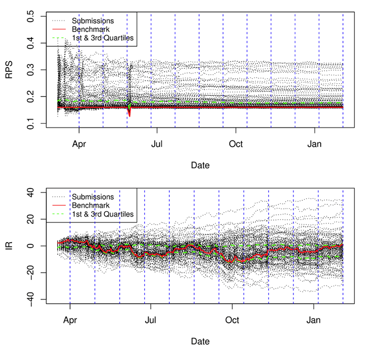
Figure 1. Daily evolution of the RPS and IR scores of the participating teams ^[1]

Among the 163 teams included in the global leaderboard, 38 (23.3%) provided more accurate forecasts than the benchmark, while 47 (28.8%) constructed better portfolios, and 11 (6.7%) achieved both higher IR and RPS scores. It is also interesting to note that, as shown in Figure 4, only three teams outperformed the benchmark’s forecasts in all 12 months of the competition, and none outperformed the benchmark's investment decisions. One team achieved higher IR scores in 11 months, and three teams in nine months. Figure 1 graphs the daily evolution of the RPS and IR scores of the 163 teams in the leaderboard. When it comes to RPS, teams perform either slightly better or considerably worse than the benchmark throughout the competition. On the contrary, the IR performance graph shows a wide range of distributions both upwards and downwards from the benchmark, indicating that a number of teams perform either significantly better or significantly worse than the benchmark, with the majority of the teams reporting lower IR scores. As shown in the above statistics and Figure 1, it was particularly difficult in practice to consistently outperform the benchmark, despite the simple forecasting and investing approaches employed by the benchmark.

Through this competition, the organizers sought to verify the hypotheses that were known in a diversity of financial fields. A total of 10 hypotheses, ranging from the efficient-market hypothesis (EMH) to the collective intelligence hypothesis, were identified, and I will share some of the key hypotheses^[1]. To reach accurate conclusions about the hypotheses, the teams whose submissions are identical to the benchmark were excluded, and then teams were selected and analyzed according to the criteria used in the hypotheses.

1. Hypothesis 1: The efficient market hypothesis will hold for the majority of teams, but it will not be the case for the top teams.

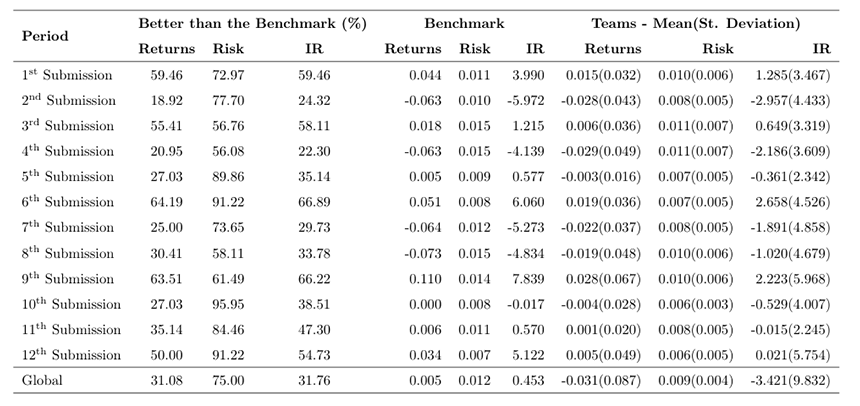
Figure 2. Statistics summarizing the performance of the benchmark and the teams (mean and standard deviation)
in terms of returns, risk, and IR across the 12 submission points and in total^[1]

Figure 2 summarizes the performance of the benchmark and the teams in terms of returns, risk, and IR across the 12 submission points individually and in total. Although the vast majority of the teams (75%) have managed to construct less risky portfolios than the benchmark, only 31% have realized higher returns and IR. Moreover, it is observed that the percentage of teams that outperformed the benchmark was usually higher when the benchmark return was positive, meaning that many teams adopted a directional bias. Therefore, it is not surprising that, overall, the benchmark did better than the ”average” team. But it is also found that some teams managed to beat the market by a significant margin. In terms of “Global” scores where the benchmark realized an IR of 0.453, the teams reported a score of −3.421 ± 9.832. In other words, assuming a normal distribution, about 16% of the teams (with a standard deviation higher than the mean) have managed to score an IR higher than 6.411, which should be regarded as a significant improvement.

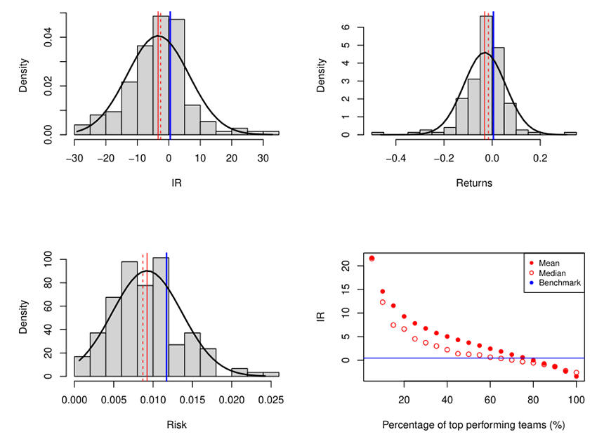
Figure 3. Distribution of IR, returns, and risk of the 148 teams whose submissions were not identical to the benchmark ^[1]

Our team (LAIR) achieved an IR of over 20. Figure 3 clearly shows that the EMH holds true for the great majority of teams, but not for the top-performing teams. In alignment with Figure 1, it indicates that while the mean and median performance of the teams is worse than the benchmark, a small number of teams achieved strongly high IR values, recording an impressive rate of return of about 30%. It is also evident that the improvements in terms of IR grow exponentially as we move from the worse to the top performing teams. At the same time, the performance of the teams is rather symmetric around the mean, indicating that more than one fourth of the teams realized losses that exceeded 7%, with the biggest loss reaching up to 46%.

1. Hypothesis 2: There will be a small group of participants who clearly outperform both in terms of forecast accuracy and investment decisions.

The average IR and RPS scores were -3.087 and 0.179, respectively, while the medians of said scores were -1.473 and 0.162. Among the participating teams, 75 (46.3%) managed to outperform the average submission, both in terms of forecast accuracy and portfolio returns, and 41 (25.3%) to outperformed the median submission. It is indicated that only a small group of participants clearly outperformed the average and the median submissions. Also, 19 of the 75 teams (and five of the 41 for the median) report negative returns, while the average forecast accuracy improvement is less than 10% (and less than 4% for the median). At the same time, the maximum accuracy improvement is 12.7% for the average submission and 3.7% for the median submission. The number of out-performing teams is even smaller when the benchmark is used as a point of reference. Specifically, only 11 teams report better IR and RPS scores than the benchmark, and although notable improvements can be identified in the investment track, forecast accuracy improvements do not exceed 2.2%. In this context, the hypothesis turns out to be true.

1. Hypothesis 3: There will be a weak link between the ability of teams to accurately forecast individual rankings of assets and risk-adjusted returns on investment, with the magnitude of this link increasing in accordance with team rankings.

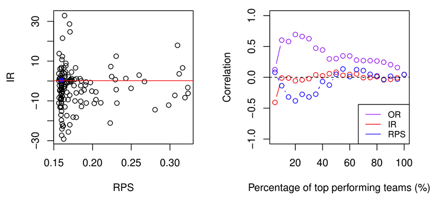
Figure 4. Correlation between IR and RPS (left), and correlation between IR and RPS, reported for various percentages of top-performing teams
(figures produced by considering OR (=overall), IR, and RPS) ^[1]

To evaluate this hypothesis, we first need to compute “r”, the correlation coefficient between IR and RPS. When the complete set of teams is considered, no connection is identified between the two variables (r = 0.04), as shown in Figure 4. Nevertheless, since the M6 was a duathlon competition, it should be the case that the top performing teams according to the OR have managed to achieve relatively high scores in terms of IR and RPS. Figure 4 confirms this hypothesis to some extent, indicating that teams of higher OR tend to build more efficient portfolios and produce more accurate forecasts at the same time. However, this link is weak as it is maximized (r = 0.7) for the top 20% of the teams but it vanishes when more than 40% of the teams are considered. Moreover, it turns out that there is no association (r = 0.12) between the two measures for the top 5% of the teams, meaning that the teams that submitted the best forecasting submissions did not perform similarly well in terms of investment decisions. The latter finding is confirmed when the same correlation analysis is conducted, but this time the teams are ranked according to their IR and RPS scores instead of OR. As shown in Figure 4, the top performing teams in the forecasting track build relatively inefficient portfolios on average (negative or close to zero coefficients), while the top performing teams in the investment decisions challenge have submitted forecasts of various accuracy levels (zero or negative).

Additionally, the following hypothesis was validated: Team portfolios will be riskier than can be theoretically justified by their forecasts. For this purpose, two variables were employed: the average number of invested assets and the average absolute investment weight per asset. As their descriptions imply, the first variable measures concentration in terms of the number of assets involved in the constructed portfolios (more assets, lower concentration, and risk), while the second in terms of capital invested per asset (larger investment weights, higher concentration, and risk). Results of measuring the correlation between the two concentration proxy variables and RPS, identified small negative correlations (r = −0.05), confirming that, in general, the risks taken by the teams cannot be justified by the accuracy of their forecasts.

1. Hypothesis 4: Top performing teams in the investment challenge will construct their portfolios using assets that they can forecast more accurately.

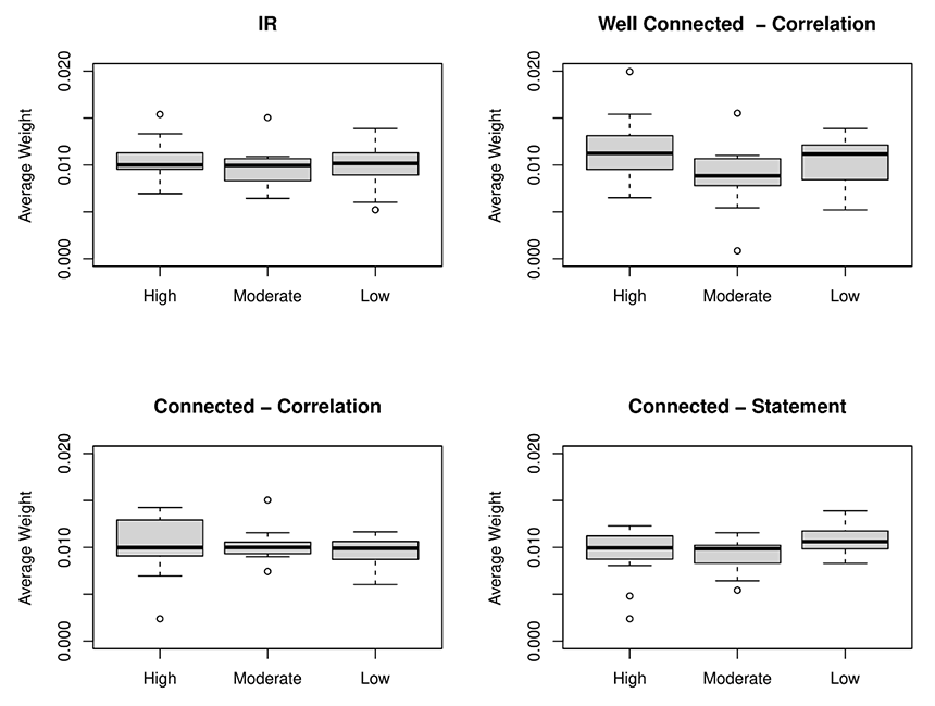
Figure 5. Distributions of average investment weights per RPS range. Analyzed for the top 15 teams of the competition in four categories.
 (“connected” refers to cases where it is assumed that there is a relationship between IR and RPS)^[1]

It was confirmed earlier that the top performing teams in the investment decision challenge did not necessarily perform similarly well in the forecast challenge. For this hypothesis, we group forecasts into three classes based on RPS scores, namely “high”, “moderate” and “low”, and then compare the average investment weights of the assets in which corresponding teams invested. If the distributions of high and low classes turn out to be significantly different, with the high class being high in weight and the low class being low, it would mean that Hypothesis 4 is true. Figure 5 presents the distribution of the investment weights for the teams selected according to different criteria. The intensity of connection was assessed based on how high the correlation between IR and RPS is. IR, correlation between IR and RPS, and answers at submission were used as the criteria. The top teams according to the IR seem to have decided their investment weights regardless of forecasts, and in the case that they are connected, there is a difference in distribution, but it is hard to say that the difference is statistically significant. In the case of the teams who said that they take both into consideration, they showed higher average investment weights for the low class. From these findings, it can be concluded that Hypothesis 4 does not hold true.

1. Hypothesis 5: Team rankings based on information ratios will be different from rankings based on returns or rankings based on the volatility of portfolio returns (risk).

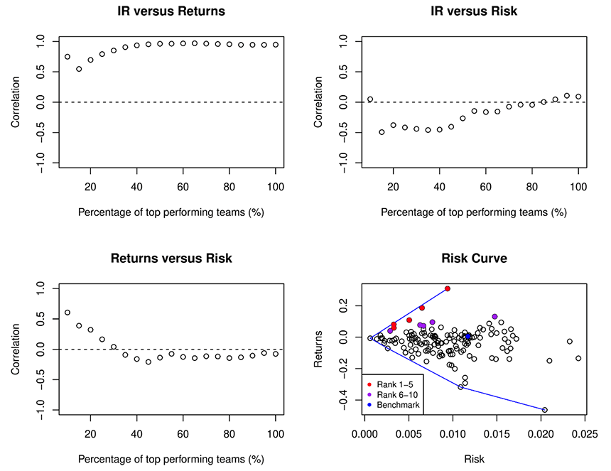
Figure 6. IRGraphs showing correlations between IR and returns, IR and risk,
and returns and risk based on the performance of participating teams^[1]

As seen in Figure 6, the correlation between risk and return was low on average and moderate for the top performing teams. There was a very strong correlation between IR and returns, but it got weaker and weaker towards the top teams. Based on this, it is hard to say that taking risks always guarantees high returns. IR and risk tended to have a weaker negative correlation towards the top teams, but they didn't correlate much for the top-tier teams. This hypothesis is true because returns and risk showed completely different patterns. The graph on the bottom right of Figure 6 shows that the top teams are achieving the highest returns on lower risks.

1. Hypothesis 6: As teams will be highly confident in the accuracy of their forecasts, forecasts will be less dispersed and have smaller variance than observed in the data.

This hypothesis is meant to verify individual teams’ certainty for outcomes. For example, if you are certain that your forecasts are accurate, you will assign one (1) to one rank for an asset, so that its ranking will not deviate into any of the other 80 rankings. In other words, we would expect that for very low assessed probabilities (near zero) the relative frequency of the outcomes would be higher than the assessed probabilities, and for very high assessed probabilities (near one) the relative frequency of the outcomes would be lower than the assessed probabilities (see, for example, Lichtenstein et al., 1982).

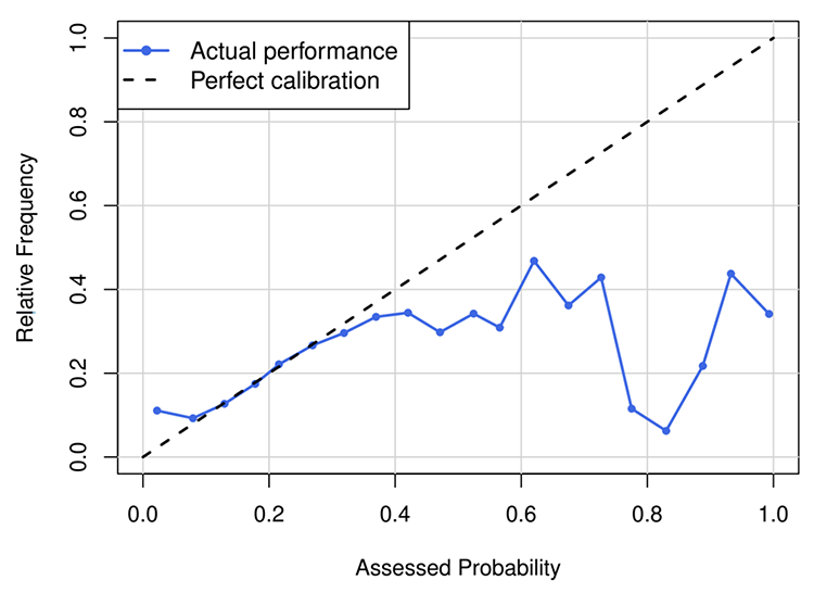
Figure 7. Relationship between assessed probability and relative frequency^[1]

Most of the participants did not perform very well in the forecasting challenge. The graph below presents the forecast results of the teams using a calibration curve, which plots relative frequency of outcomes against assessed probabilities of those outcomes. The dotted diagonal line represents perfect calibration, and the solid line shows the actual performance. For assessed probabilities higher than 0.3, the relative frequency is less than the assessed probability, substantially so as assessed probability increases. On the contrary, for very low assessed probabilities, the relative frequency is higher than that assessed. This leads to the conclusion that extreme probabilities show the teams’ overconfidence in the outcomes. Additionally, an analysis of the outcomes of the top 10 teams found that they did not assign high probabilities of 0.7 or higher. Taken together, this hypothesis can be said to be true.

1. Hypothesis 7. Averaging forecast rankings (investment weights) across all teams (excluding the worst performing teams) for each asset will yield rankings (weights) that outperform those of the majority of the teams.

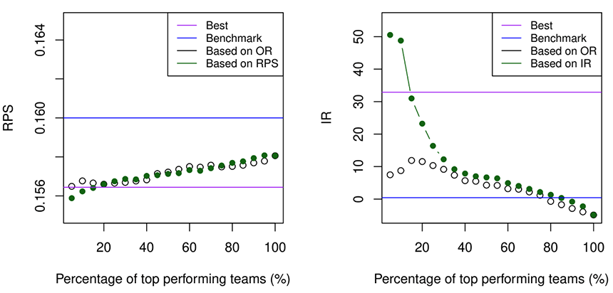
Figure 8. The graphs above show the results of combining team submissions (selected based on team performance)
and assessing the outcomes against RPS and IR (performance based on RPS, IR, and OR)^[1]

This hypothesis is about collective intelligence. We could obtain better outcomes when we applied the average of the outcomes for the majority of the teams for each asset, excluding the teams with poor outcomes. As you can see in Figure 8, averaging the forecasts of the teams according to the RPS resulted in superior performance over the benchmark, and combining the top 20% outcomes yielded better results than the best performing team. However, combining the top teams based on the OR, which considers both tracks, produced a performance close to the best, but not better. Measured against IR, the combination of the top 80% and combinations of higher-ranking teams beat the benchmark, and the combination of the top 15% performed almost 170% better than the best. On the contrary, OR-based results were steadily rising towards the top rank but started to fall at the very top. Taken together, the results show that collective intelligence works effectively.

Among the analysis results of the main hypotheses, there were expected results, but unexpected results were also confirmed. In summary, it was once again confirmed that it is very difficult to make accurate forecasts in most cases. Of course, there were teams that did better than the benchmark, but given that the perfect score is 0 and the benchmark is 0.16, the fact that the best performance scored 0.14-5 is a good indication of the limitations of forecasting. In other words, figuring out how to get an RPS of 0.1 or lower is really a big challenge. In the IR section, about 60% exceeded the usual 7%, and the lowest was a return rate of -46%. In addition, less than one third of the teams have managed to outperform the benchmark. Moreover, a very small group of participants have managed to outperform the market consistently. It is impressive that none of the teams has achieved higher IR than the benchmark in all 12 months of the competition and only four have beat the market in eight months or longer. Our team was one of the four teams, taking fourth place overall. According to an analysis of the results, it should be particularly noted that the our team performed better when the benchmark was bearish, which means that the other teams failed to construct their portfolios precisely by including short selling as a means to respond when losing value.

Also, with regard to the finding that the correlation between forecasts and investment performance is weak, we have researched and developed forecast-based techniques to consider both of the tracks. An additional finding is that collective intelligence tends to be right. However, in reality, it is difficult to get other investors' portfolios; therefore, we can assume that we will get better outcomes if we can incorporate information that indirectly reflects them. Lastly, rather than sticking to one strategy consistently, employing and changing strategies to respond to changes in the market has led to better outcomes. Approaches such as distribution shift, out-of-distribution (OOD) detection, and anomaly, which are widely discussed in the field of AI, have been effective in adapting to market changes, yielding good outcomes.

Since market participants rarely expose their strategies, the results shared in this competition are highly valuable. Although the approximately 200 participating teams may not represent the entire market, understanding the strategies they employ and the results they achieve is crucial in a competitive environment. We will incorporate these factors into AI to better forecast, explain, and solve optimization problems.

2. The Future of Time Series Forecasting

Photo 2. The future of forecasting and the M6 competition conference
ⓒhttps://mofc.unic.ac.cy/

Next, I'd like to share some of the issues that have been discussed in academia and industry about research trends and outlooks for AI-based forecasting problems. We looked into what kinds of forecasting problems Big Tech companies selling forecasting technologies, such as Meta and Google, as well as universities are working on and how they are approaching solutions. In this post, I will focus on the issues that were mentioned the most.

First of all, the topic that was talked about the most is Large Language Models (LLMs). None of the teams were using an LLM for forecasting yet, but most of them were considering a plan to use them. There have been many attempts to build a model particularly based on news, due to the fact that unstructured text data can be factored into forecasting. You can use an LLM in a wide variety of situations through instruction tuning, going beyond simply analyzing emotions. You can receive changes in conditions in the form of text inputs, configure simulations to allow outcomes, that is, forecast values to change, and develop your model gradually through user feedback. The LLM technology can be used to improve forecasting performance itself, but it also enables you to explain forecasting outcomes. As forecasting technology continues to advance, there has been an opinion that the ability to explain is required when we move from the stage of using forecasts as a reference to the stage of direct use. The participants shared the same concern that, if we just have forecasting values, it is difficult to apply them easily, even if the accuracy is 100%. We easily related to this as we had a similar concern. However high the accuracy may be, forecasting alone cannot solve everything. We learned that this is not something that happens only to LG, but to everyone who works to apply AI to actual business processes. Interestingly enough, we realized that it is a complex problem that requires us to consider not only algorithms but also users’ psychological responses.

In this respect, we see LLMs as a useful tool to overcome this problem. The competition of scale triggered by LLM technology is also impacting time series forecasting. On the other hand, there were expectations and outlooks for large-scale forecasting. While the majority of the previous studies have focused on how to better forecast a single time series, there were voices calling for the need to conduct research on large-scale time series forecasting in the future. Just as many problems in the field of language were solved using super-large models and large volumes of data in ways that would not have been possible before, they believe that something similar would happen in time series forecasting. It follows from this that, if we start to forecast a lot of time series data, we can bring about different outcomes and new research topics, unlike dealing with only 100 or 1000 time series. We could see at the conference that Big Tech companies were already making such attempts and that they saw a lot of potential in LLM. As the LG AI Research Institute is also dealing with super-large models, we also see the potential that we could continue to take on challenges at the global level in the field of time series in tandem with this trend.

Furthermore, the participants shared diverse directions for solving forecasting problems. First of all, we found that attempts were being made to actively utilize synthetic data as well as observed data. Recently, an academic society held a competition for time-series generative AI models that could incorporate desired characteristics. The underlying reason for these attempts is that time series data has a smaller amount of information than images and languages. Not only is the data relatively small in size, but it is also difficult to use other background knowledge than numbers when evaluating results. As an alternative that can fill these gaps, many forecasting experts are placing great importance on synthetic data. The use of synthetic data may be a good way to increase the amount of information, even if it is not the type of data that is recorded by observation, as long as it can help improve the accuracy of forecasts. Moreover, in order to forecast even for cases where new prices that have not been available before, such as lithium, continue to be released, you cannot rely on just using past data. You should make sure that various time series incorporating different scenarios be learned together with other types of data to respond to extreme OOD issues.

In the same context, the participants also discussed one of the problems that everyone faces: how to handle missing values. Unlike data meant for schools or experiments, it is often the case that real-world data cannot be learned without preprocessing due to missing values or inconsistent recording frequencies, unless it is recorded by a machine set to record data periodically. Therefore, such methods as imputation and interpolation are used to solve problems with missing values, or statistical models are used to fill in the gaps. But AI is a better candidate to fill the gaps, and there have also been discussions on models that can be trained to fill in the gaps in ways fit for a given purpose. This is an area that has been researched for a long time, but it requires a lot of tuning to be effective. At the conference, we learned through these trials and errors in the real world of business that it is possible to configure a model with a structure generalized to some extent and that it is a process that must be applied to improve performance.

Current forecasting practices and many tips were shared, but there was one common question: "What is a good forecast?" In general, a good forecast indicates a high forecast accuracy. In reality, however, forecast accuracy is not reflected, as it is, in the use of forecasts by working-level personnel and business decision-making. Although advances in AI technology have made it possible to some extent to forecast using complex data, many experts believe that aiming solely for accuracy is not sufficient. In the field of demand forecasting, in order to produce high-accuracy forecasts, we need to not only consider the accuracy of each region and brand but to also pay attention to probabilistic forecasts, stability, and explainability. These are all major factors in forecasting, but one that is easy to miss in practice is stability. Stability has to do with costs, rather than maintaining a consistently high level of accuracy. For example, suppose that you make one forecast for a certain point in the future six months before the point in time and another three months before. If the forecast value six months ago was 100 and that of three months ago is 110, there is a difference of 10 for the same point in time. This difference changes production and distribution plans associated with the forecast, which in turn increases costs. These cost issues may be negligible for small companies, but they can be a reason for large companies involved in global logistics to hesitate to use AI forecasts. At this conference, various measures were proposed to solve these problems. One of them is to add a stability term to loss so that stability is considered during the learning process. This improved loss is applicable regardless of models, and the purpose is to take into account the forecasts that have been made earlier. Therefore, the advantage is that you don't suddenly get an outcome that is significantly different from the previous forecast trends and that you can enjoy the momentum effect. On the other hand, it was expected that it would not work very well in cases where rapid variations could occur, but actual results show that it has some effect despite rapid changes. This is particularly convincing as the effects of the outcomes were verified by the demand data, M3 and M4. We found a clue to solve some of our problems as LG AI Research has been conducting demand forecasting for its affiliates and has also been tackling the same issues.

As such, forecasting has areas that cannot be assessed simply by forecasting errors. Therefore, forecasting problems should not be viewed only by focusing on forecasts themselves but as part of the decision-making process. Defining a good forecast based solely on 'errors' may not be optimal in terms of decision-making. It is interesting to note that a similar conclusion was drawn from the interviews with forecasters from many Big Tech companies. That is, it is time to move away from talking about simple accuracy. It was also suggested that the purpose of the forecasting process was not to make an accurate forecasting but to allow working-level personnel to discuss whether all the factors necessary for the forecasting had been considered. The conclusion is that after these processes pass, in the future, forecasting is likely to become a function that is naturally and inherently included in all aspects, rather than being some special technical skill. To make it happen, we need to think about what makes a good forecast and what model should be used by going backwards from the final decision that needs to be made. Therefore, the LG AI Research's Data Intelligence Lab, which has been conducting a range of AI research projects to interpret, forecast, and optimize complex data, also intends to further advance technologies that are effective in business decision-making, in addition to its current research on forecasting models.