[NeurIPS 2023] Multimodal Generation for Audio and Music

1. Introduction

Art creation using AI was a hot topic at NeurIPS 2023, with many papers, company booths, and workshops showcasing the feat. A variety of tech companies demonstrated interesting research and services, particularly in audio and music generation areas. For example, Google DeepMind’s AI music tool “Lyria” and Meta’s “Audiobox” garnered a lot of attention.

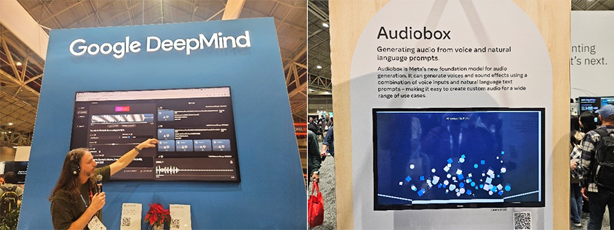
Image 1. Google DeepMind’s Lyria (left), Meta’s Audiobox (right).

Google DeepMind's Lyria creates 30-second songs that reflect a specific artist’s voice and musical style and can be used in YouTube Shorts. You can also use a text prompt to change the style of a music sample that Lyria provides while keeping the musical elements intact. At their booth, Jesse Engel of the Magenta team, which designs artistic learning AI algorithms at Google, gave a demo of his voice being converted into a drum sample while beatboxing.

Meta’s Audiobox is a comprehensive model that can perform text-to-speech, text-to-audio, text-to-audio infilling, text-to-effect, vocal restyling, and more. The combination of audio input and natural language text prompts makes it easy to create a variety of audio and sound effects.

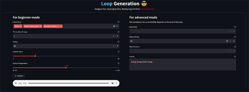
Image 2. The Interface for Music Loop Generation^[14]

LG AI Research’s Data Intelligence (DI) Lab also published a paper titled “The Interface for Symbolic Music Loop Generation Conditioned on Musical Metadata^[14]” This research was demonstrated during NeurIPS 2023’s workshop session through active interaction with music researchers. LG AI Research’s interface receives metadata related to music, such as instruments, tempo, average pitch, and average duration, and generates a MIDI loop consisting of four measures. This enables music creators and researchers to work more efficiently and creatively.

As shown above, AI can be used to generate a wide variety of audio and music without the need for specialized knowledge. Recently, researchers have been working to further utilize data from other modals, such as text, to control the signals. Now we’ll cover the evolution of technologies and technologies underlying multimodal generation research, such as text-to-image and text-to-music, and related research that were presented at NeurIPS 2023.

2. Multimodal Generation Overview

Most multimodal generation research follows a framework consisting of a prior that connects different modals to an encoder/decoder structure that compresses large-space data, as shown in the figure below.

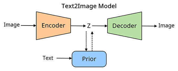
Image 3. Multimodal Generation Framework (e.g. Text-to-Image)

First, an autoencoder is learned to obtain compressed data representation. Next, a powerful prior is configured to generate through a condition like text. In the inference phase, sampling starts from the condition and is restored to the original domain using the learned decoder. It is similar in structure to VAE, but the differences are that 1) it is designed to maximize resilience by separating the learning of the autoencoder and prior in two stages, and 2) it is designed to use the learned prior to sample in a meaningful space. Next, let’s touch upon the VQ-VAE family of methods for compressing large-space data with an autoencoder, which provides a discrete representation of the data.

3. Discrete Representations

In the real world, data is represented in an infinite, continuous space. However, a near-perfect representation can be achieved by combining finite chunks of meaning. For example, the smallest unit of meaning can be an object in an image, a word in a language, or a phoneme in audio. If the data in each domain can be represented through a combination of objects, words, and phonemes, the number of data units needed to be generated is reduced to a finite number. This next section will explore the core principles of VQ-VAE, the leading model for learning discrete representations, as well as VQ-GAN, which improves the performance of VQ-VAE, and the residual vector quantizer, which is on its way to becoming the standard technology for discrete representation in the audio domain.

3.1 VQ-VAE

VQ-VAE^[1] is a family of autoencoders that compress and restore data. It represents each element of compressed data as a finite number of codes by finding each element in a trainable dictionary $e$ ($e\in {{\mathrm{ℝ}}^{}}^{K\times D},$ $K$ is the number of codes in the dictionary, $D$ is the embedding dimension corresponding to each code).

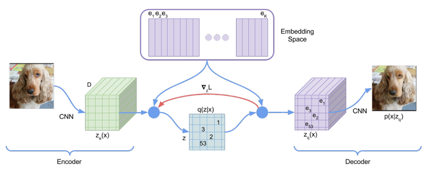
Image 4. VQ-VAE Overview^[1]

Using Image 4 as an example, let’s say a compressed image$z_e\left(x\right)$ has dimensions (width, height, channel) of $8\times 8\times 10$, $K$ in the dictionary is 512, and $D$ in the dictionary is 10. In such a case, the compressed image can have codes via quantization, and each code can have an integer index from 0 to 511. To restore the image represented by the combination of codes to the original data space, we simply need to find the embedding that corresponds to the index in the dictionary (the image of is restored to image) and send it to the decoder.

For learning, reconstruction loss is used to reduce the difference between the original data and the restored data. Likewise, the dictionary is updated using L2 loss or a moving average to avoid moving too far away from the embedding space. Here, as the process of looking up the dictionary cannot be differentiated, learning is performed by simply skipping this part during the backpropagation process. This method is similar to the straight-through gradient estimation (ST estimation) method for calculating gradients in discrete latent variable models. In a similar vein, a paper that theoretically proved that ST estimation is a first-order approximation of the actual gradients was selected for oral presentation^[2] at NeurIPS 2023.

3.2 VQ-GAN

VQ-GAN^[3]adds patch-based adversarial loss to VQ-VAE loss to learn perceptually rich code. This loss divides the data recovered from the decoder into patches (compressed to the desired number of patches using a CNN discriminator in the actual implementation) and learns to discriminate whether each patch is real or fake. Compared to VQ-VAE, VQ-GAN shows better performance on perceptual-related metrics (e.g., FID, FAD) with fewer codes in the dictionary and can be utilized for both image or audio spectrograms depending on the data domain^{[3, 4]}.

3.3 Residual Vector Quantizer (RVQ)

A sufficient number of dictionary values must be set to fully represent data as a discrete representation. For example, for raw audio, no matter how many hundreds of times you compress with an autoencoder, the value of $K$ will increase by powers of 2 depending on the compression bitrate that is targeted. To improve and solve this, RVQ^[5] iteratively performs quantization over multiple dictionaries, passing the residuals from quantization to the next dictionary.

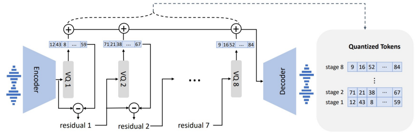
Image 5. Process of RVQ^[6]. To express one compressed frame,
a total of 8 codes corresponding to the frame are used from 8 dictionaries.

Say the value of $K$ needed to sufficiently represent the data in VQ-VAE is $2^{80}$. You can use 8 RVQs to reduce the value of $K$ needed for one dictionary to the level of $2^{80/8}$ Additionally, the quantizer that passes first plays the most important role in reconstruction.

3.4 Improved RVQGAN

Introduced at NeurIPS 2023, the improved RVQGAN^[9] borrows many ideas from well-performing vocoders (spectrogram to waveform inversion models, e.g. HiFiGAN^[10], BigVGAN^[11]) to improve reconstruction performance with a 90-times higher compression rate. As the compression model was learned at 44.1kHz for data from various sources such as speech, music, and environmental sound, it aims for a universal audio compression model. Let’s take a closer look at the additional ideas applied in improved RVQGAN in addition to the basic VQ-VAE, VQ-GAN, and RVQ explanations that we touched on earlier.

3.4.1 Periodic Activation Function

Activation functions such as LeakyReLU have poor extrapolation because they do not fully reflect the periodicity of the signal. The improved RVQGAN utilizes the snake activation used in BigVGAN to inject a periodic inductive bias into the decoder.

3.4.2 Mitigating Codebook Collapse

The VQ-VAE family model has a problem with codebook collapse, in which certain codes are rarely used during training. The problem has been previously solved by initializing the embedding of the dictionary with K-means or applying randomized restarts to the embedding of infrequently used code. The improved RVQGAN applies a kind of regularization to the code embedding (PCA to generate lookup embedding, L2-normalization) so that the code can be used uniformly without K-means or randomized restarts.

3.4.3 Quantize Dropout Rate

In the paper “SoundStream: An End-to-End Neural Audio Codec^[5],” a quantizer dropout was applied to cover various bitrates with one model. As the bitrate is determined by the number of dictionaries used for RVQ, this method randomizes the number of dictionaries used per sample. The improved RVQGAN improves the reconstruction quality to near-optimal at full bandwidth by probabilistically applying a quantizer dropout per sample.

3.4.4 Discriminator Design

Adversarial training was run with the appropriate discriminator for the audio domain. It used the multi-period waveform discriminator used in existing Vocoder research. In addition, a complex STFT discriminator was additionally applied at various timescales to reflect phase information.

3.4.5 Loss Functions

Loss functions of reconstruction loss (multi-scale spectral L1 loss), adversarial loss (multi-period waveform loss, complex STFT loss, L1 feature matching loss), and VQ-VAE loss (commitment loss) were also used. Unlike existing research, it was possible to secure good performance without adaptively setting the loss weight.

3.4.6 Balanced Data Sampling

The improved RVQGAN requires preprocessing to resample data from various sources, fixing 44.1kHz audio as input. The frequency limit at which the model could recover was checked via experiment and was found to be around the average sample rate of the dataset. To improve this, the batch was forced to include at least one sample that met the desired Nyquist frequency (22.05 kHz) and balanced sampling was applied to ensure that data from different sources were mixed.

The author verified the validity of each design choice through an ablation study and confirmed that it showed good reconstruction quality with a compression ratio 90 times higher than the existing audio compression model. The improved RVQGAN is expected to be utilized as a good foundation model for audio representation, compression, and generation research as it learns to cover data from various sources and sample rates.

4. Prior

Once the data has been expressed in a discrete representation or code by a VQ-VAE family of models, it can be linked with data in another modal (e.g., tokenized text) to learn a prior. As they are expressed as a sequence of tokens, autoregressive models from the GPT family are often used.

Discrete diffusion models can also be utilized^{[7, 8]}. However, if you compress the data using RVQ as described in 3.3 (Residual Vector Quantizer [RVQ]), the length of the sequence that needs to be learned by the prior increases by a factor depending on the number of times RVQ is applied. For example, in Image 5, 8 RVQs were applied, which means 8 residual codes were used to represent one compressed frame.

At NeurIPS 2023, research was introduced that proposed an efficient way to arrange RVQ-compressed residual code in a text-to-music task^[12]. First, EnCodec^[13] was used with RVQ to compress the audio into residual discrete code. The author introduced four patterns (flattening, parallel, coarse first, and delay) for arranging compressed code as shown in the Figure below, and experimentally verified their generation performance.

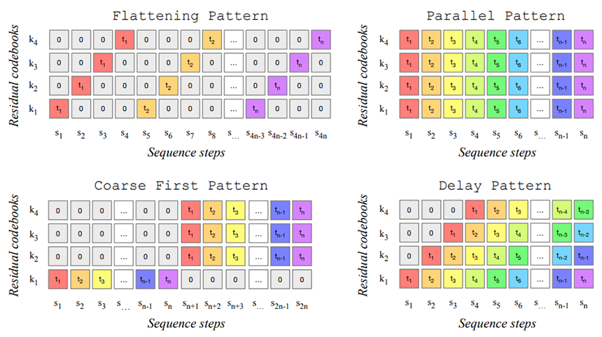
Image 6. Four Patterns for Arranging RVQ Code^[12].
Assuming that RVQ is applied 4 times, quantization is indicated by ${\mathit{k}}_{\mathbf{1}}\mathbf{.}\mathbf{.}\mathbf{.}{\mathit{k}}_{\mathbf{4}}$ in the order of application.

In Image 6, 1) the flattening pattern flattens all residual codes into a 1D sequence, so the length of the sequence increases by 4 times. 2) For parallel patterns, the length of the sequence is maintained regardless of the number of RVQ applications because the transformer input embedding layer adds all the residual codes of the same sequence step. 3) As mentioned before, the first passing quantizer ($k_1$) contains the most important information, so the coarse first pattern generates all the important information and loses the less important information. 4) The delay pattern is designed to alternately arrange the residual code of different steps so that the information of a specific code is not lost. The code sequence of each pattern was learned with the next token prediction method through utilization of transformer models of 300M, 1.5B, and 3.3B in size, and then restored to audio using EnCodec’s decoder.

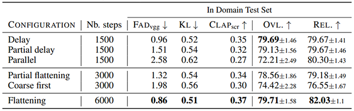
Image 7. Comparison of Music Generation Performance According to RVQ Code Arrangement Patterns^[12].
FAD, KL, and CLAP use pre-trained models to evaluate the fidelity of music,
and OVL. and REL. evaluate music quality and relevance to text through human evaluation.

As a result, the flattening pattern performs the best in terms of generating music but suffers from the problem of generating long code. As an alternative, the delay pattern shows good generation performance while maintaining fewer steps.

5. Conclusion

This post explored the evolution of multimodal generation research with a focus on discrete representations. It also introduced an improved RVQGAN that compresses audio more effectively than research that was previously presented at NeurIPS 2023, as well as a paper that proposed an efficient way to arrange residual code in text-to-music. I believe that the advancement of Transformer, which allows us to easily and powerfully handle discrete data, has been a major catalyst for the development of multimodal research, making it easier to model the relationship between multiple modals.

The LG AI Research DI Lab is conducting research on multimodal generation, with the ultimate research goal of generating real sound on a song-by-song basis by inputting various modes. As a first step toward achieving this goal, we are currently focusing on MIDI generation research that reduces the data representation space for generating music and enables artists to easily edit generated music. At LG AIResearch’s DI Lab, we strive to perform research in the realm of auditory art to enable anyone to discover and express their own artistic identity.